Peak Analysis
1. Peak Profiling
Wrapper Function
The peak_profiling() function runs the full peak
profiling workflow in one call. It performs peak calling from bedGraph
input and, if enabled, applies downstream annotation including genomic
distribution summaries, pathway annotation, and TFBS enrichment. For
users who prefer fine-grained control over parameters, please refer to
the detailed parameter settings below.
Parameters
| Parameter | Type | Default | Description | Example |
|---|---|---|---|---|
bedgraph_path |
character | — | Vector of bedGraph file paths used as input for peak calling. Each file is treated as one sample/target for downstream peak calling and annotation. | bedgraph_path = c("sampleA.bedgraph", "sampleB.bedgraph") |
out_dir |
character | "./" |
Output directory for all pipeline results, including peak calling
output and the genomic_distribution,
pathway_annotation, and TFBS_enrichment
subdirectories generated during annotation.
The directory is created automatically if it does not exist.
|
out_dir = "./peak_profiling_results/" |
ref_genome |
character | "hg38" |
Reference genome used throughout peak calling and all downstream
annotation steps (genomic distribution, pathway annotation, and
TFBS enrichment). Supported options are "hg38" and
"mm10".
|
ref_genome = "mm10" |
min_cov |
numeric | 2 |
Minimum coverage threshold used to pre-filter bedGraph intervals before peak calling. | min_cov = 5 |
auc_top_pct |
numeric | 0.1 |
Top percentage (by area under the curve) of candidate regions retained during peak calling. | auc_top_pct = 0.2 |
qvalue_cutoff |
numeric | 0.05 |
FDR-adjusted p-value (q-value) cutoff used to call significant peaks during peak calling. | qvalue_cutoff = 0.01 |
fc_cutoff |
numeric | 2 |
Minimum fold-change threshold used to call significant peaks during peak calling. | fc_cutoff = 1.5 |
apply_annotation |
logical | TRUE |
Whether to run the downstream annotation steps (genomic
distribution, pathway annotation, and TFBS enrichment) after
peak calling. If FALSE, only peak calling is performed.
|
apply_annotation = FALSE |
plot |
logical | TRUE |
Whether to generate visualizations (genomic distribution plots,
pathway bubble plot, and TFBS enrichment heatmap) in each
annotation step. Only used when apply_annotation = TRUE.
|
plot = FALSE |
1A. Peak Calling
The peak_calling() function identifies enriched genomic
signal blocks (peaks) directly from one or more bedGraph files by
scanning per-chromosome read coverage, merging contiguous non-zero
segments into blocks, estimating local background using proportional
flanking windows, and applying an enrichment test with BH
correction.
What this function does:
This function reads aligned sequencing reads coverage tracks from bedGraph files and processes each file independently. For each chromosome, it extracts contiguous non-zero coverage intervals and merges adjacent intervals into larger “signal blocks” when the current interval starts exactly at the previous interval end.
For every block, the function calculates a block-level signal AUC (sum of coverage over the block) and estimates a local background AUC by extending upstream and downstream flanks with a length proportional to the block size (4.5× the block length on each side; bounded by chromosome edges). The background region includes the block itself plus both flanks, so the enrichment test is performed by comparing the block AUC against the total AUC in the expanded local neighborhood.
Candidate peaks are then determined in three steps:
Optional mean coverage pre-filter (
min_cov): Blocks whose mean coverage (auc / length) falls belowmin_covare discarded before statistical testing. This step targets “wide-and-shallow” blocks — long blocks with signal density near the background floor that can otherwise accumulate large total AUC purely by length, despite carrying no real enrichment signal. Removing them here also keeps them from inflating the denominator of the downstream multiple-testing correction.Statistical testing: Enrichment significance is evaluated using a binomial tail probability, where the total “trials” correspond to the local background AUC and the success probability is the length fraction (
block_length / bg_length). If the AUC values are non-integer (e.g. from normalized coverage tracks), a Poisson approximation is used instead. The resulting p-values are adjusted with BH correction to obtain q-values. Blocks passing both the statistical significance threshold (qvalue_cutoff) and the fold change threshold (fc_cutoff) are retained as candidate peaks.AUC post-filter (
auc_top_pct): Among the statistically significant candidate peaks, only those whose AUC falls within the specified top fraction are retained. This removes low-signal peaks that passed the significance thresholds but carry weak absolute enrichment, and is conceptually analogous to the top-fraction threshold used in SEACR.
Peaks are then exported in narrowPeak format
(.narrowPeak) with MACS2-compatible columns
(signalValue, pValue, qValue,
peak), compatible with rtracklayer::import()
and standard peak analysis tools.
Parameters
| Parameter | Type | Default | Description | Example |
|---|---|---|---|---|
bedgraph_path |
character vector | — | Vector of bedGraph file paths. Each bedGraph is processed independently (file-level parallelism), and the function returns a named list of output BED file paths. | bedgraph_path = c("C1_H3K27ac.bedGraph", "C1_H3K4me3.bedGraph") |
out_dir |
character | "./" |
Output directory to save peak BED files. Created recursively if it does not exist. | out_dir = "./peaks" |
ref_genome |
character | "hg38" |
Reference genome build used to define standard chromosomes and chromosome lengths.
Supported values: "hg38", "mm10".
Chromosome naming style (UCSC vs NCBI) is auto-detected from the first bedGraph
(presence/absence of chr prefix) and applied to the genome object.
|
ref_genome = "mm10" |
min_cov |
numeric | 2 |
Minimum mean coverage (auc / length) required for a block to be considered as a candidate peak. This filter is applied before statistical testing and removes "wide-and-shallow" blocks — long blocks with signal density near the background floor that can otherwise accumulate large total AUC purely by length, despite carrying no real enrichment signal.
|
min_cov = 2 |
qvalue_cutoff |
numeric | 0.05 |
BH-adjusted q-value cutoff for peak significance filtering. | qvalue_cutoff = 0.01 |
fc_cutoff |
numeric | 2 |
Fold-change cutoff for peak filtering. Fold change is computed as mean signal in the block divided by mean
signal in the local background neighborhood:
(auc / block_length) / (bg_auc / bg_length).
|
fc_cutoff = 3 |
auc_top_pct |
numeric | 0.01 |
Fraction of blocks to retain based on AUC ranking prior to statistical testing. Only blocks whose AUC falls within the top fraction are considered as candidate peaks; e.g., The default value 0.01 retains only the top 1% of blocks by AUC.
|
auc_top_pct = 0.01 |
Parameter tuning guidance:
The default values
min_cov = 2andauc_top_pct = 0.1are intentionally conservative. Some wide-and-shallow blocks may still pass through under these settings.If the peaks will feed into downstream differential analysis (DA), keep these conservative defaults to retain a sufficiently large candidate pool. An overly small candidate set can compromise the statistical power and reliability of DA results (e.g., unstable normalization and dispersion estimates). Tighter filtering on
covorauccan then be applied after DA to further narrow down the peak set to higher-confidence regions.If the peaks will be used directly for downstream analysis such as annotation or visualization, consider raising
min_cov(and/or tighteningauc_top_pct) according to sequencing depth, since there is no subsequent DA step to compensate for residual low-confidence peaks.
Output Files
The function generates the following output file(s) for each input
BAM in the specified out_dir:
- Peak BED file -
<pair>_peaks.narrowPeak-
<pair>refers to the BAM filename without extension -
The output is a BED file with a header, compatible with common
peak-processing tools, and contains the following columns:
-
chrom: Chromosome name -
chromStart: 0-based start coordinate -
chromEnd: 1-based end coordinate (BED end; exclusive semantics are not enforced and correspond to the block end) -
name: Peak identifier in the formatchr:start-end -
score: Integer score derived from-log10(q_value)(scaled and capped at 1000) -
strand:. -
signalValue: Enrichment fold change (fc) -
pValue:-log10(p_value) -
qValue:-log10(q_value) -
peak: Relative summit position to peak start, computed as the midpoint of the highest-signal bedGraph interval(s) within the block- All intervals within the block sharing the maximum signal value are identified as summit candidates.
- If these candidates are contiguous (form a single uninterrupted plateau), the summit spans from the start of the first to the end of the last candidate interval.
- If these candidates are scattered (separated by lower-signal intervals), the candidate closest to the geometric center of the block is selected as the summit, avoiding an artificial span across intervening low-signal gaps.
-
The reported
peakvalue is the midpoint of the selected summit interval(s), expressed as an offset fromchromStart.
 </li>
 <li><code>length</code>: Peak length in base pairs (<code>chromEnd - chromStart</code>)</li>
 <li><code>auc</code>: Total signal (area under the curve) within the peak block</li>
 <li><code>cov</code>: Mean coverage within the peak block, computed as <code>auc / length</code></li>
-
-
Note: this file extends the standard 10-column narrowPeak format with
three additional columns (
length,auc,cov). Tools that strictly validate column count or type against the official narrowPeak spec (e.g.rtracklayer::import()without an explicitextraColsargument) may fail to parse it; tools that read columns positionally or via flexible BED readers (e.g.data.table::fread,bedtools, IGV) are unaffected.
-
| chrom | chromStart | chromEnd | name | score | strand | signalValue | pValue | qValue | peak | length | auc | cov | |
|---|---|---|---|---|---|---|---|---|---|---|---|---|---|
| 1 | chr1 | 924754 | 925901 | chr1:924754-925901 | 1000 | . | 3.44102741224937 | 844.120728079697 | 843.762092600299 | 890 | 1147 | 3065 | 2.67218831734961 |
| 2 | chr1 | 960217 | 961971 | chr1:960217-961971 | 1000 | . | 5.27827863925953 | 2074.0773448214 | 2072.70019010491 | 382 | 1754 | 4391 | 2.50342075256556 |
| 3 | chr1 | 1304439 | 1306480 | chr1:1304439-1306480 | 1000 | . | 6.05496021352685 | 2712.72145876509 | 2710.87146159186 | 1574 | 2041 | 4940 | 2.4203821656051 |
| 4 | chr1 | 2231096 | 2232510 | chr1:2231096-2232510 | 1000 | . | 4.63098591549296 | 1335.48254184973 | 1334.72224204123 | 142 | 1414 | 3288 | 2.32531824611033 |
| 5 | chr1 | 3771354 | 3772564 | chr1:3771354-3772564 | 1000 | . | 4.26711560044893 | 1397.26861845056 | 1396.46233020521 | 593 | 1210 | 3802 | 3.14214876033058 |
| … | … | ||||||||||||
Example BED output showing peak-calling results for the
H3K4me1-H3K4me1 pair in sample C1 from the
test dataset.
Example Usage
library(multiEpiCore)

# ===== Test Data =======
bg_base_dir <- "./bedgraph"
out_dir <- "./peak"
min_cov <- 2
auc_top_pct <- 0.1

bg_dirs <- list.dirs(bg_base_dir, full.names = TRUE, recursive = FALSE)

for (bg_dir in bg_dirs) {
  sample <- basename(bg_dir)
  sample_out <- file.path(out_dir, sample)
  bg_paths <- list.files(path = bg_dir, pattern = "\\.bedGraph$", recursive = FALSE, full.names = TRUE)
  peak_calling(
    bedgraph_path = bg_paths,
    out_dir = sample_out,
    min_cov = min_cov,
    auc_top_pct = auc_top_pct
  )
}
1B. Peak-level Pathway Annotation
The peak_pathway_annotation() function provides an
automated workflow for performing pathway enrichment annotation on peak
BED files across multiple targets. It converts each BED file into a
GRangesList, runs rGREAT-based pathway
enrichment against MSigDB Hallmark gene sets, saves per-target
enrichment tables, and optionally generates a combined bubble plot
summary.
Parameters
| Parameter | Type | Default | Description | Example |
|---|---|---|---|---|
peak_path |
character | — |
Vector of BED file paths containing peak regions.
Each BED file is treated as one target, and the target name is inferred
from the file basename after removing pattern
(e.g., stripping _peaks.narrowPeak).
The BED files must contain at least three columns:
chromosome, start, and end.
|
peak_path = c("CTCF_peaks.narrowPeak", "H3K27ac_peaks.narrowPeak") |
out_dir |
character | "./" |
Output directory where pathway enrichment results will be saved. The directory is created automatically if it does not exist. Per-target TSV tables and the optional bubble plot PDF are written here. | out_dir = "./peak/sampleA" |
ref_genome |
character | "hg38" |
Reference genome used to select the TSS annotation database for rGREAT.
Supported options are "hg38" and "mm10".
|
ref_genome = "mm10" |
msigdb_collection |
character | "H" |
MSigDB collection abbreviation. Common values: "H" (Hallmark, 50 curated biological states), "C2" (curated gene sets including KEGG and Reactome), "C5" (GO gene sets). See msigdbr::msigdbr_collections() for the full list. |
"C2" |
pattern |
character | "_peaks.\\narrowPeak$" |
Regular expression used to remove suffix text from each BED filename when constructing target names. This must match the naming convention of your peak files; otherwise, target names may be incorrect or non-unique. | pattern = "\\.narrowPeak$" |
plot |
logical | TRUE |
Whether to generate a combined bubble plot summarizing pathway enrichment
across all targets.
If FALSE, only per-target TSV tables are generated.
|
plot = FALSE |
Output Files
All output files are saved to the specified out_dir:
- Per-target pathway enrichment table -
pathway_annotation_<target>.tsv
- rGREAT enrichment results for each target peak set (one BED file)
- Contains the following columns:
pathway: Name of the enriched MSigDB Hallmark gene set (with the “HALLMARK_” prefix removed).hits_region: Number of input peak regions assigned to genes belonging to this pathway.fold: Fold enrichment of observed region-gene associations compared to the genomic background expectation.p: Raw p-value from the enrichment test assessing whether the association is statistically significant.padj: Multiple-testing adjusted p-value (FDR) correcting for testing across many pathways.hits_gene: Number of unique genes in this pathway that are linked to at least one input peak.
| pathway | hits_region | fold | p | padj | hits_gene |
|---|---|---|---|---|---|
| HEME_METABOLISM | 751 | 2.34242482729004 | 0 | 0 | 158 |
| IL6_JAK_STAT3_SIGNALING | 279 | 2.1539487647391 | 0 | 0 | 49 |
| P53_PATHWAY | 667 | 1.96477997521663 | 0 | 0 | 143 |
| UNFOLDED_PROTEIN_RESPONSE | 314 | 1.88450359297116 | 0 | 0 | 75 |
| TGF_BETA_SIGNALING | 267 | 1.78440015179855 | 0 | 0 | 42 |
| DNA_REPAIR | 278 | 1.71262469023883 | 0 | 0 | 90 |
| ESTROGEN_RESPONSE_EARLY | 828 | 1.69192498116218 | 0 | 0 | 154 |
| ESTROGEN_RESPONSE_LATE | 665 | 1.66254073916161 | 0 | 0 | 151 |
| ADIPOGENESIS | 530 | 1.64575217378315 | 0 | 0 | 145 |
| HYPOXIA | 734 | 1.61320155249418 | 0 | 0 | 140 |
| TNFA_SIGNALING_VIA_NFKB | 792 | 1.58554145852615 | 0 | 0 | 152 |
| XENOBIOTIC_METABOLISM | 450 | 1.56279143172028 | 0 | 0 | 127 |
| UV_RESPONSE_UP | 443 | 1.54357603879619 | 0 | 0 | 107 |
| IL2_STAT5_SIGNALING | 712 | 1.53461386388768 | 0 | 0 | 139 |
| MTORC1_SIGNALING | 505 | 1.49494285184175 | 0 | 0 | 123 |
| APICAL_JUNCTION | 551 | 1.463680066491 | 0 | 0 | 139 |
| APOPTOSIS | 475 | 1.48104653987793 | 3.33066907387547e-16 | 9.79608551139844e-16 | 110 |
| MITOTIC_SPINDLE | 529 | 1.36376400697203 | 4.01345623401994e-12 | 1.11484895389443e-11 | 142 |
| PI3K_AKT_MTOR_SIGNALING | 302 | 1.49192024874113 | 3.21923598889384e-11 | 8.4716736549838e-11 | 70 |
| MYOGENESIS | 508 | 1.31864023785508 | 9.69003322026651e-10 | 2.42250830506663e-09 | 141 |
| MYC_TARGETS_V2 | 119 | 1.82974169254377 | 1.20143017756646e-09 | 2.86054804182492e-09 | 36 |
| REACTIVE_OXYGEN_SPECIES_PATHWAY | 103 | 1.77523750310684 | 6.06994279284123e-08 | 1.37953245291846e-07 | 34 |
| G2M_CHECKPOINT | 513 | 1.26492214857928 | 1.23927521800127e-07 | 2.69407656087232e-07 | 136 |
| ANDROGEN_RESPONSE | 330 | 1.33614385753243 | 2.39605753793448e-07 | 4.9917865373635e-07 | 75 |
| INTERFERON_GAMMA_RESPONSE | 444 | 1.26193664345416 | 1.04498334296821e-06 | 2.08996668593642e-06 | 109 |
| MYC_TARGETS_V1 | 320 | 1.29514823159424 | 4.42162588376593e-06 | 8.50312669954987e-06 | 117 |
| OXIDATIVE_PHOSPHORYLATION | 340 | 1.27782170145938 | 6.7021178460358e-06 | 1.24113293445107e-05 | 132 |
| PEROXISOME | 227 | 1.34919819212654 | 8.78569769868776e-06 | 1.56887458905138e-05 | 67 |
| GLYCOLYSIS | 493 | 1.21410566576122 | 1.33914178344074e-05 | 2.30886514386335e-05 | 139 |
| COAGULATION | 274 | 1.2900533590942 | 2.61656722224668e-05 | 4.36094537041113e-05 | 81 |
| E2F_TARGETS | 340 | 1.22929930562074 | 0.000113631696623262 | 0.000183276930037519 | 123 |
| PROTEIN_SECRETION | 243 | 1.21740811782978 | 0.00152880417435064 | 0.00238875652242287 | 58 |
| COMPLEMENT | 438 | 1.13378486167835 | 0.00491815778703741 | 0.00745175422278396 | 126 |
| INFLAMMATORY_RESPONSE | 499 | 1.11258543831093 | 0.00935157469816006 | 0.0137523157325883 | 123 |
| INTERFERON_ALPHA_RESPONSE | 158 | 1.18824427654253 | 0.0184387753694073 | 0.0263411076705819 | 49 |
| APICAL_SURFACE | 142 | 1.19709034950041 | 0.0197614340616903 | 0.0274464361967921 | 31 |
| NOTCH_SIGNALING | 99 | 1.23636420287506 | 0.0222803736236655 | 0.0301086130049534 | 20 |
| ALLOGRAFT_REJECTION | 359 | 1.09140387222255 | 0.0517507656437572 | 0.0680931126891543 | 101 |
| KRAS_SIGNALING_DN | 455 | 1.07232300390841 | 0.0706418972348002 | 0.0905665349164105 | 117 |
| CHOLESTEROL_HOMEOSTASIS | 155 | 1.12700521636616 | 0.0753616524855787 | 0.0942020656069734 | 47 |
| WNT_BETA_CATENIN_SIGNALING | 140 | 1.1286634877976 | 0.0839096466534721 | 0.102328837382283 | 30 |
| FATTY_ACID_METABOLISM | 279 | 1.08475876599981 | 0.0920066254830114 | 0.109531697003585 | 91 |
| ANGIOGENESIS | 104 | 1.12332164952526 | 0.128663088630856 | 0.149608242594018 | 18 |
| HEDGEHOG_SIGNALING | 145 | 0.969022723736511 | 0.659136328916236 | 0.749018555586632 | 30 |
| SPERMATOGENESIS | 258 | 0.90177989643402 | 0.957419784368706 | 1 | 79 |
| UV_RESPONSE_DN | 554 | 0.924360737401476 | 0.972326175648468 | 1 | 95 |
| BILE_ACID_METABOLISM | 188 | 0.853630810616856 | 0.988205830454095 | 1 | 61 |
| KRAS_SIGNALING_UP | 508 | 0.870884862971025 | 0.999415085430068 | 1 | 119 |
| PANCREAS_BETA_CELLS | 81 | 0.685957113608895 | 0.999876069754364 | 1 | 26 |
| EPITHELIAL_MESENCHYMAL_TRANSITION | 442 | 0.697646781527174 | 1 | 1 | 112 |
Note: This table shows the pathway enrichment annotation results for peaks from C1 sample.
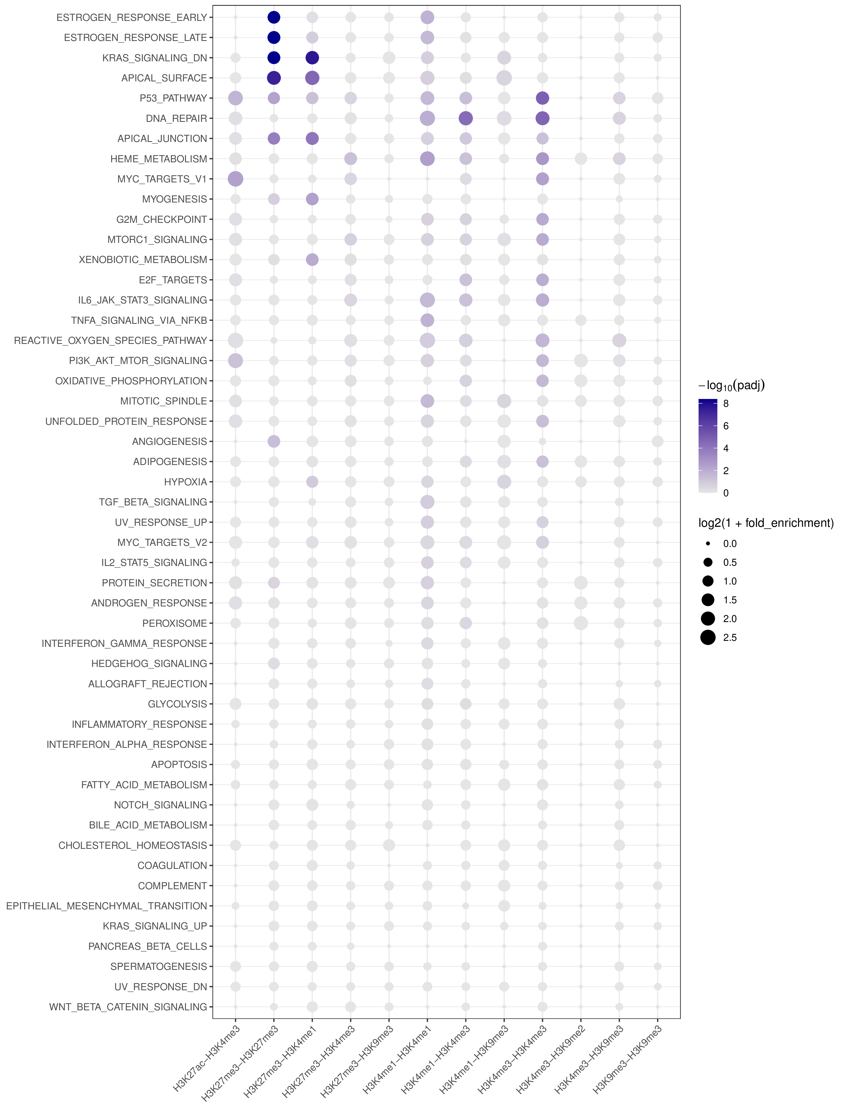
- Cross-target bubble plot -
pathway_annotation.pdf(whenplot = TRUE)
- A combined summary visualization across all targets and pathways
- x-axis: target (BED-derived name)
- y-axis: pathway
- point color: capped
-log10(padj)for visual stability - point size:
log2(1 + fold_enrichment)
Example Usage
library(multiEpiCore)

# ===== Test Data =======
pk_base_dir <- "./peak"
pk_dirs <- list.dirs(pk_base_dir, full.names = TRUE, recursive = FALSE)

for (pk_dir in pk_dirs) {
  sample <- basename(pk_dir)
  peak_paths <- list.files(path = pk_dir, pattern = "\\.narrowPeak$", recursive = FALSE, full.names = TRUE)
  pathway_out <- file.path(pk_dir, "pathway_distribution")
  peak_pathway_annotation(
    peak_path = peak_paths,
    out_dir = pathway_out
  )
}
1C. Peak-level Genomic Distribution
The peak_genomic_distribution() function performs
genomic feature annotation for peak BED files and quantifies their
distribution across regulatory element categories. Each peak set is
converted into genomic ranges and annotated against selected reference
resources such as gene features, cCRE elements, ChromHMM chromatin
states, and repeat elements, followed by optional visualization of
distribution patterns.
Parameters
| Parameter | Type | Default | Description | Example |
|---|---|---|---|---|
bed_path |
character | — |
Path(s) to input BED files, or a directory containing BED files.
Each BED file is treated as one target, and target names are extracted
from filenames using pattern.
|
c("CTCF_peaks.narrowPeak", "H3K27ac_peaks.narrowPeak") |
out_dir |
character | "./" |
Output directory for annotation results. Results for each annotation type and target are saved here. | "./distribution_results" |
pattern |
character | "_peaks\\.narrowPeak$" |
Regular expression used to remove suffix text from each BED filename when constructing target names. This must match the naming convention of your peak files; otherwise, target names may be incorrect or non-unique. | pattern = "\\.narrowPeak$" |
distributions |
character vector | c("genic", "ccre") |
Annotation types to compute.
Supported options are "genic", "ccre",
"chromhmm", and "repeat".
At least one annotation type must be specified.
|
c("genic", "ccre", "repeat") |
ref_genome |
character | "hg38" |
Reference genome version used for annotation.
Supported options are "hg38" and "mm10".
|
"mm10" |
ref_source |
character | "knownGene" |
Gene annotation source for genic-based annotation.
Supported options are "knownGene" (UCSC)
and "GENCODE".
|
"GENCODE" |
mode |
character | "nearest" |
Method used to assign peaks to genomic features.
"nearest" assigns each peak to the closest feature,
while "weighted" assigns annotations proportionally
based on overlap length.
|
"weighted" |
plot |
logical | TRUE |
Whether to generate visualization plots summarizing genomic distribution across annotation categories. | FALSE |
- Annotation types available:
"genic": Gene structural features - Promoter, 5’ UTR, Exon, Intron, 3’ UTR"ccre": Candidate cis-Regulatory Elements - dELS, pELS, PLS, CA-H3K4me3, CA-CTCF, CA-TF, TF, CA"chromhmm": Chromatin states - Acet, EnhWk, EnhA, PromF, TSS, TxWk, TxEx, Tx, OpenC, TxEnh, ReprPCopenC, BivProm, ZNF, ReprPC, HET, GapArtf, Quies"repeat": Repetitive elements - SINE, LINE, LTR, Retroposon, RC, DNA, Satellite, Simple_repeat, Low_complexity, rRNA, tRNA, snRNA, scRNA, srpRNA, RNA, Unknown- For detailed description of each annotation category, see the Annotation page
- Annotation assignment methods:
"nearest": Each genomic region is assigned to its closest feature (by distance to feature center)"weighted": Each region is proportionally assigned to overlapping features based on overlap lengthnearestmode is faster and simpler;weightedmode provides more accurate representation for regions spanning multiple features
Output Files
The function generates the following output files in the specified
out_dir: 1. Composition tables -
{genic/ccre/chromhmm/repeat}_distribution.tsv - .tsv tables
summarizing the percentage composition of various annotations - Row:
cluster lables - Col: annotations states - Values represent the
proportion (%) of genomic regions assigned to each state within a
cluster
- Genic distribution
| Promoter | 5’ UTR | Exon | Intron | 3’ UTR | other | |
|---|---|---|---|---|---|---|
| H3K27me3-H3K4me1 | 13.55 | 1.39 | 7.16 | 46.07 | 2.37 | 29.46 |
| H3K27me3-H3K4me3 | 25.88 | 3.98 | 9.22 | 38.76 | 2.14 | 20.02 |
| H3K27me3-H3K9me2 | 8.96 | 0.96 | 5.57 | 49.88 | 2.05 | 32.58 |
| H3K27me3-H3K9me3 | 10.61 | 1.04 | 6.17 | 47.40 | 2.06 | 32.72 |
| …… | ||||||
| H3K9me3-H3K9me3 | 6.79 | 0.70 | 4.30 | 45.85 | 1.41 | 40.95 |
- cCRE distribution
| dELS | pELS | PLS | CA-H3K4me3 | |
|---|---|---|---|---|
| H3K27me3-H3K4me1 | 50.47 | 13.57 | 8.13 | 2.40 |
| H3K27me3-H3K4me3 | 35.62 | 21.39 | 21.62 | 2.01 |
| H3K27me3-H3K9me2 | 39.89 | 9.36 | 4.06 | 2.66 |
| H3K27me3-H3K9me3 | 40.86 | 9.89 | 5.74 | 3.17 |
| …… | ||||
| H3K9me3-H3K9me3 | 26.82 | 5.78 | 3.51 | 4.54 |
| CA-CTCF | CA-TF | TF | CA | other | |
|---|---|---|---|---|---|
| H3K27me3-H3K4me1 | 2.43 | 0.86 | 2.18 | 4.41 | 15.55 |
| H3K27me3-H3K4me3 | 1.50 | 0.47 | 1.62 | 2.99 | 12.79 |
| H3K27me3-H3K9me2 | 2.79 | 0.78 | 2.58 | 6.06 | 31.82 |
| H3K27me3-H3K9me3 | 2.82 | 0.82 | 2.64 | 5.86 | 28.21 |
| …… | |||||
| H3K9me3-H3K9me3 | 2.98 | 0.77 | 3.02 | 6.78 | 45.79 |
Note: These tables show the genomic distribution results for peaks from the C1 sample.
- Cmposition bar plot -
{genic/ccre/chromhmm/repeat}_distribution.pdf- Stacked horizontal bar plot showing ChromHMM chromatin state distribution across clusters
- X-axis: Percentage (0-100%)
- Y-axis: Cluster labels (top to bottom)
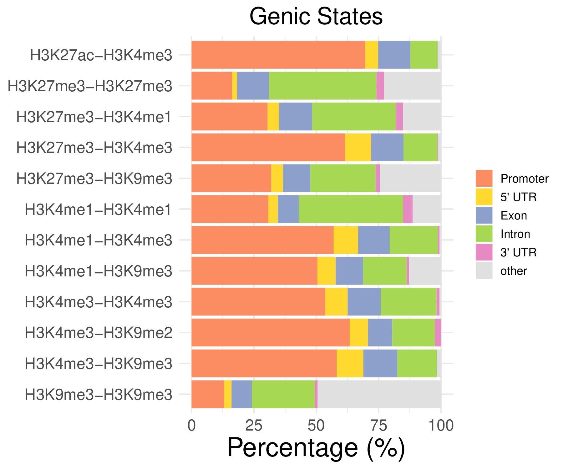
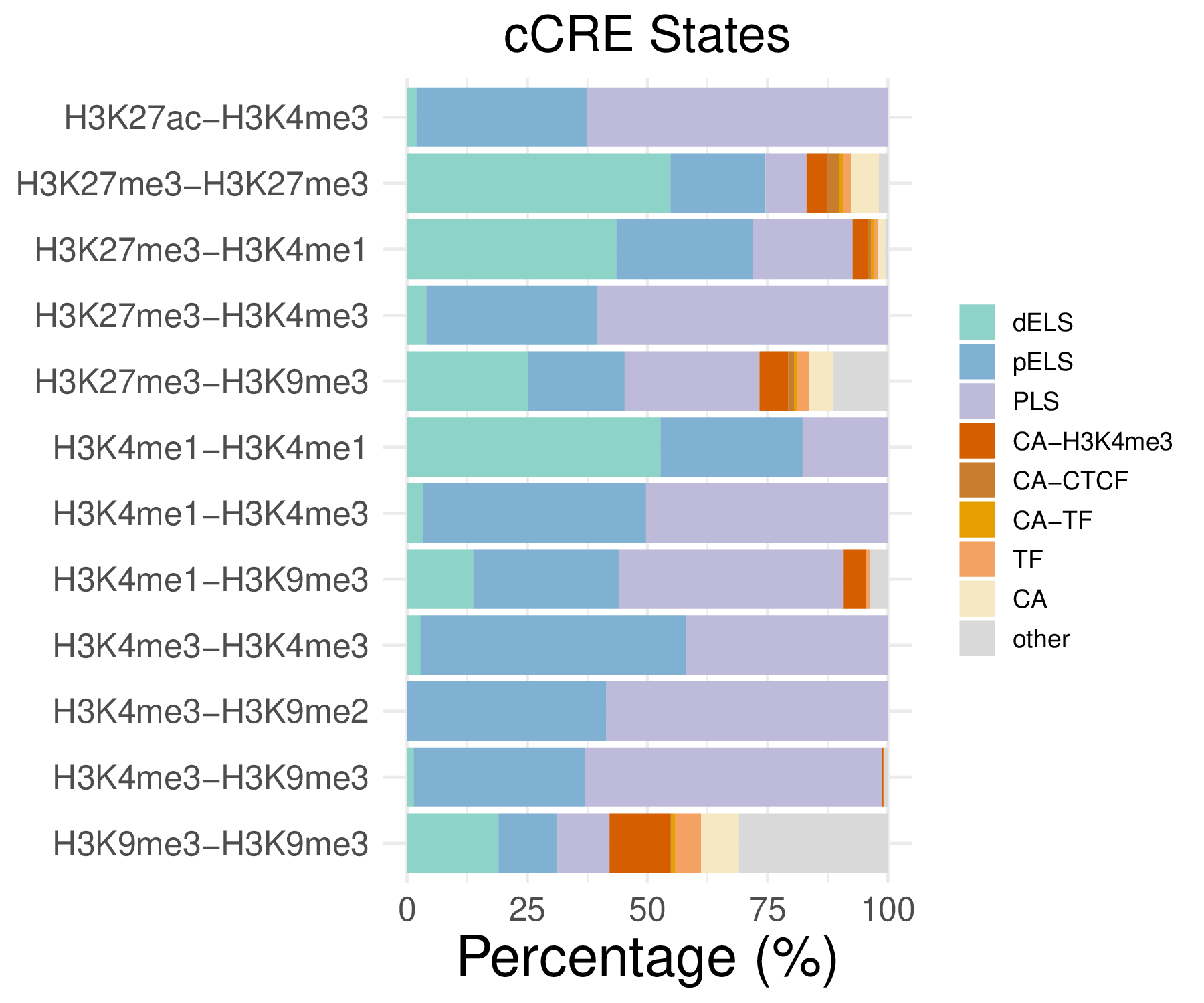
Note: These figurs show the genomic distribution results for peaks from the C1 sample.
Example Usage
library(multiEpiCore)

# ===== Test Data =======
pk_base_dir <- "./peak"
pk_dirs <- list.dirs(pk_base_dir, full.names = TRUE, recursive = FALSE)

for (pk_dir in pk_dirs) {
  sample <- basename(pk_dir)
  peak_paths <- list.files(path = pk_dir, pattern = "\\.narrowPeak$", recursive = FALSE, full.names = TRUE)
  genomic_out <- file.path(pk_dir, "genomic_distribution")
  peak_genomic_distribution(
    peak_path = peak_paths,
    out_dir = genomic_out
  )
}
1D. Peak-level TFBS Enrichment Analysis
The peak_TFBS_enrichment() function performs
transcription factor binding site (TFBS) enrichment analysis for peak
files against matched genomic background regions. Peak summits are
resized to a fixed window and compared to control regions generated from
the reference genome, followed by enrichment testing and optional
heatmap visualization of the top-ranked TFs across targets.
Parameters
| Parameter | Type | Default | Description | Example |
|---|---|---|---|---|
peak_path |
character | — |
Vector of peak file paths (e.g., narrowPeak files).
Each file is treated as one target, and the target name is inferred
from the file basename after removing pattern.
Peaks are read and anchored on the summit position rather than the
geometric center of the region.
|
peak_path = c("CTCF_peaks.narrowPeak", "H3K27ac_peaks.narrowPeak") |
out_dir |
character | "./" |
Output directory where control regions (all_controls.bed),
per-target enrichment TSV tables, and the optional heatmap are saved.
The directory is created automatically if it does not exist.
|
out_dir = "./TFBS_results/" |
ref_genome |
character | "hg38" |
Reference genome used for generating matched control regions and for
TFBS annotation. Supported options are "hg38" and
"mm10".
|
ref_genome = "mm10" |
ref_source |
character | "knownGene" |
Gene annotation source used for control region generation.
Supported options are "knownGene" (UCSC knownGene)
and "GENCODE" (GENCODE gene models).
|
ref_source = "GENCODE" |
pattern |
character | "_peaks\\.narrowPeak$" |
Regular expression used to strip suffix text from each peak filename when constructing target names. This must match the naming convention of your peak files; otherwise, target names may be incorrect or non-unique. | pattern = "\\.narrowPeak$" |
control_rep |
integer | 1 |
Multiplier for control region generation, defining the ratio of control
regions to target regions. Must be at least 1.
For example, control_rep = 2 generates twice as many
control regions before deduplication.
|
control_rep = 3 |
regions |
integer | 800 |
Size in base pairs to which all query and control regions are resized, centered on the peak summit (for query regions) or region center (for control regions after overlap reduction). | regions = 500 |
plot |
logical | TRUE |
Whether to generate a TFBS enrichment heatmap across all targets.
If FALSE, only the per-target enrichment TSV tables are
generated.
|
plot = FALSE |
plot_n_top |
integer | 20 |
Number of top-ranked TFs to display in the enrichment heatmap.
Only used when plot = TRUE.
|
plot_n_top = 30 |
seed |
integer | 42 |
Random seed used to ensure reproducible generation of matched control regions. | seed = 123 |
Output Files
- Matched control regions -
all_controls.bed- BED file containing all matched control regions used as background for TFBS enrichment analysis
- Regions are combined across clusters and de-duplicated to avoid redundant counting
- Cluster-level TFBS enrichment table -
TFBS_enrichment_<cluster_label>.tsv
- Per-cluster transcription factor binding site enrichment results
- Includes odds ratio, p-value, FDR, and hit counts for each TF motif
| feature | target_hit | control_hit | target_off | control_off | odds_ratio | pvalue | odds_ratio_se | FDR |
|---|---|---|---|---|---|---|---|---|
| MAX | 207 | 1720 | 30 | 7758 | 30.2597566549319 | 1.30766409855477e-114 | 0.194359710167716 | 4.04068206453423e-112 |
| HDAC2 | 178 | 1159 | 59 | 8319 | 21.384395719867 | 1.27304500305104e-105 | 0.152432018023272 | 1.96685452971385e-103 |
| RCOR1 | 160 | 926 | 77 | 8552 | 19.0322037333513 | 7.9773271042011e-98 | 0.142222922332352 | 8.21664691732713e-96 |
| EP300 | 130 | 565 | 107 | 8913 | 19.0843628060824 | 1.34064739637776e-88 | 0.137010271806922 | 1.03565011370182e-86 |
| JUND | 158 | 1052 | 79 | 8426 | 15.8967896364339 | 9.09963938278453e-88 | 0.140917145814258 | 5.62357713856084e-86 |
Note: This table shows annotation results for H3K4me1-H3K4me1 in the sample C1.
- Full TFBS enrichment heatmap -
TFBS_heatmap_all.pdf(ifplot = TRUE)- Heatmap visualization of enriched TFBS across all clusters
- Log2-transformed odds ratios with a symmetric color scale
- Rows: TFBS
- Columns: Cluster labels

- Top N TFBS heatmap -
TFBS_enrichment_top<n>.pdf(iftop_nprovided andplot = TRUE)- Heatmap showing the top N TFBS with the highest coefficient of variation across clusters
- Highlights TFBS exhibiting the greatest variability between clusters
- Uses the same log2 odds ratio color scale as the full heatmap for consistency
- Rows: TFBS
- Columns: Cluster labels
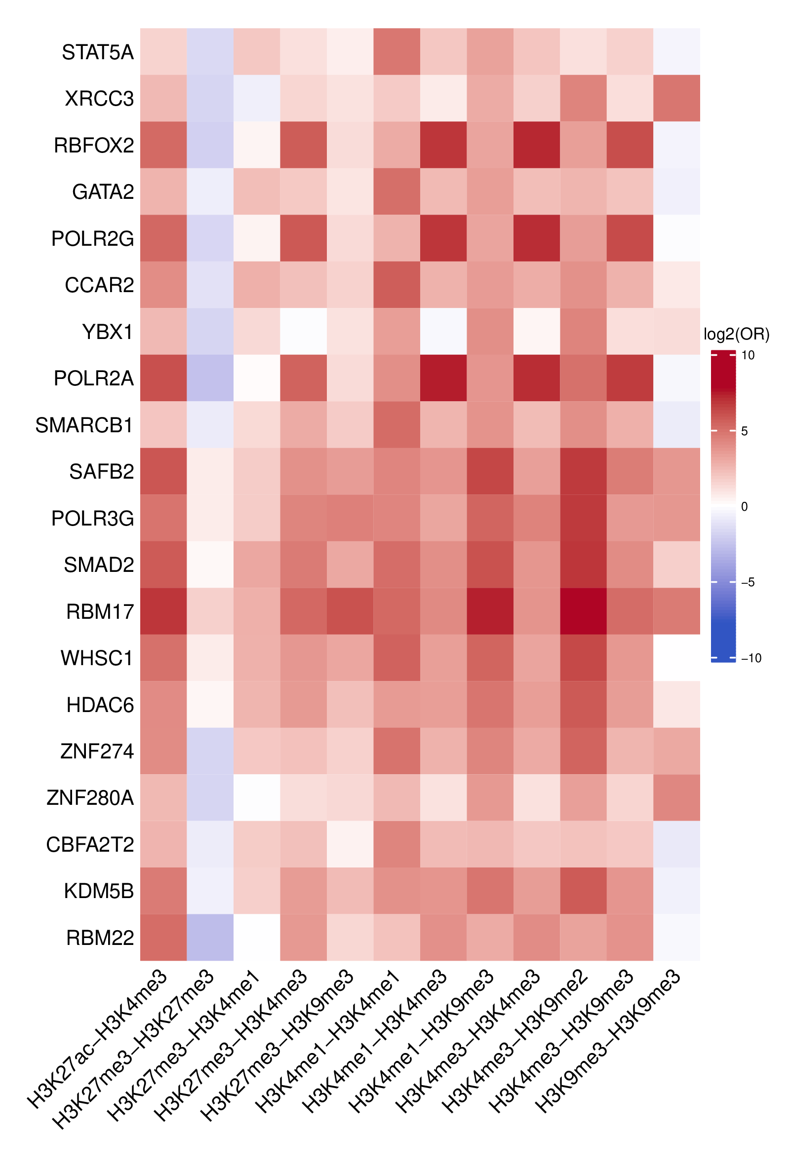
- Log2 odds ratio matrix -
odds_ratio_log2.csv(ifplot = TRUE)- Matrix of log2-transformed odds ratios for all TFBS × clusters
- Numerical data underlying the TFBS enrichment heatmap
- Rows: TFBS
- Columns: Cluster labels
- FDR matrix -
FDR.csv(ifplot = TRUE)- Matrix of FDR-adjusted p-values for all TFBS × clusters
- Same row and column order as
odds_ratio_log2.csv
Example Usage
library(multiEpiCore)

# ===== Test Data =======
pk_base_dir <- "./peak"
pk_dirs <- list.dirs(pk_base_dir, full.names = TRUE, recursive = FALSE)

for (pk_dir in pk_dirs) {
  sample <- basename(pk_dir)
  peak_paths <- list.files(path = pk_dir, pattern = "\\.narrowPeak$", recursive = FALSE, full.names = TRUE)
  TFBS_out <- file.path(pk_dir, "TFBS_enrichment")
  peak_TFBS_enrichment(
    peak_path = peak_paths,
    out_dir = TFBS_out
  )
}
2. Peak Differential Analysis
Wrapper Function
Unlike other steps in this package where each function operates across all CRF pairs simultaneously, the differential analysis here is structured per CRF pair across samples. This reflects the biological reality that each CRF pair targets a distinct genomic locus set — peak regions from different CRF pairs are not directly comparable and should never be pooled into a shared count matrix.
peak_differential_analysis() is the recommended entry
point for this step. It wraps build_peak_set() and
differential_regions_single_peak() into a single call: for
each CRF pair found consistently across all sample directories, it first
constructs a condition-aware consensus peak set, then counts fragment
overlap per sample and runs the voom-limma differential analysis.
| Parameter | Type | Default | Description | Example |
|---|---|---|---|---|
peak_dirs |
character vector | — | One directory per sample containing narrowPeak files. Must be in the same order as conditions. Each directory is scanned for files matching peak_pattern; the pair name is extracted by stripping the pattern from the filename. |
peak_dirs = c("./peak/C1", "./peak/C2", "./peak/T1", "./peak/T2") |
bam_dirs |
character vector | — | One directory per sample containing BAM files, in the same order as peak_dirs and conditions. Pair names are extracted by stripping bam_pattern from the filename; only pairs present across all BAM and peak directories are processed. |
bam_dirs = c("./bam/C1", "./bam/C2", "./bam/T1", "./bam/T2") |
conditions |
character vector | — | Condition label for each sample, in the same order as peak_dirs and bam_dirs. Each condition must have at least 2 replicates. |
conditions = c("C", "C", "T", "T") |
sample_names |
character vector or NULL | NULL |
Optional display names for each sample, in the same order as conditions. If NULL, names are auto-generated as {condition}{replicate_index}. |
sample_names = c("C1", "C2", "T1", "T2") |
ref_genome |
character | "hg38" |
Reference genome used to obtain chromosome sizes for boundary checking during tiling. Must be one of "hg38" or "mm10". Ignored when window_size is NULL. |
ref_genome = "mm10" |
out_dir |
character | "./" |
Root output directory. Consensus BED files are written to {out_dir}/peak_sets/ and differential results to {out_dir}/differential/. |
out_dir = "./results" |
bam_pattern |
character | "\\.bam$" |
Regular expression used to remove suffix text from each BAM filename when constructing target names.
This must match the naming convention of your BAM files and produce the same target names as peak_pattern;
otherwise, pair matching across peak and BAM directories will fail.
|
bam_pattern = "\\.bam$" |
peak_pattern |
character | "_peaks\\.narrowPeak$" |
Regex pattern used to scan peak_dirs and to strip the suffix when extracting pair names from filenames. |
peak_pattern = "_peaks\\.narrowPeak$" |
window_size |
integer or NULL | NULL |
Passed to build_peak_set(). If NULL, master regions are used directly. If a positive integer, regions are tiled into fixed-size windows. |
window_size = 500L |
min_support |
integer | 2 |
Passed to both build_peak_set() and differential_regions_single_peak(). Minimum number of samples within at least one condition group required to retain a region at the peak-building stage, and to pass the non-zero filter at the testing stage. |
min_support = 2 |
lfc_threshold |
numeric | 0.5 |
Minimum absolute log2 fold-change for significance. | lfc_threshold = 0.5 |
p_threshold |
numeric | 0.05 |
P-value threshold for significance. Interpreted according to p_type. |
p_threshold = 0.05 |
p_type |
character | "fdr" |
Which p-value to use for filtering: "fdr" (BH-adjusted, recommended for genome-wide analysis), "nominal" (raw p-value, suitable for pre-selected gene lists), or "bonferroni" (conservative correction). |
p_type = "nominal" |
Output Structure
{out_dir}/
├── peak_sets/
│   ├── {pair}.bed          # consensus peak set per CRF pair
│   └── ...
└── differential/
    ├── {test}_vs_{ref}_{pair}_all.tsv
    ├── {test}_vs_{ref}_{pair}_sig.tsv
    ├── {test}_vs_{ref}_summary.tsv
    ├── {test}_vs_{ref}_summary.pdf
    └── ...
Example Usage
peak_differential_analysis(
  peak_dirs  = c("./peak/C1", "./peak/C2", "./peak/T1", "./peak/T2"),
  bam_dirs   = c("./bam/C1",  "./bam/C2",  "./bam/T1",  "./bam/T2"),
  conditions = c("C", "C", "T", "T"),
  sample_names = c("C1", "C2", "T1", "T2"),
  out_dir    = "./peak",
  min_support  = 2,
  window_size  = NULL,
  lfc_threshold = 0.5,
  p_threshold  = 0.05,
  p_type       = "fdr"
)
2A. Build Peak Set
Given a set of narrowPeak files from the same target(CRF
pair) across multiple samples, build_peak_set()
function constructs a unified peak set that represents regions
consistently enriched across the cohort.
What this function does:
First, all per-sample peak intervals are pooled together. The genome
is then atomized into the smallest non-overlapping sub-intervals defined
by all peak boundaries, and each sub-interval is scored by how many
distinct samples contain it. Sub-intervals supported by fewer than
min_support samples are discarded as sample-specific noise;
the remaining sub-intervals are merged into contiguous consensus blocks
wherever they are adjacent.
- If
window_sizeisNULL, these master regions are exported directly as the final peak set (each region retains its natural variable width). - If
window_sizeis specified, each master region is divided into fixed-size windows tiled outward from the region’s center. The number of windows is ceil(region_width / window_size). For an odd number of windows, the center window is anchored at the region midpoint; for an even number, the midpoint falls at the boundary between the two central windows. Windows that extend beyond chromosome boundaries are discarded.
Parameters
| Parameter | Type | Default | Description | Example |
|---|---|---|---|---|
peak_path
|
character vector | — |
Vector of narrowPeak or BED file paths, one per sample. Each file must
contain at least three columns: chrom,
chromStart, chromEnd.
|
peak_path = c(“S1_peaks.narrowPeak”, “S2_peaks.narrowPeak”)
|
pair
|
character | — |
Output file basename (without extension). The final BED file is written
as <pair>.bed inside out_dir.
|
pair = “H3K27ac_consensus”
|
conditions
|
character vector | — |
Condition label for each sample, in the same order as
peak_path. Used together with min_support to
apply a per-group reproducibility filter.
|
conditions = c(“ctrl”, “ctrl”, “treat”, “treat”)
|
ref_genome
|
character |
“hg38”
|
Reference genome used to obtain chromosome sizes for boundary checking
during tiling. Must be one of “hg38” or
“mm10”. Ignored when window_size is
NULL.
|
ref_genome = “mm10”
|
out_dir
|
character |
“./”
|
Output directory. Created recursively if it does not exist. |
out_dir = “./peak_sets”
|
window_size
|
integer or NULL |
NULL
|
If NULL, master regions are exported directly. If a
positive integer, each master region is tiled into fixed-size windows of
this width. Regions narrower than window_size are skipped.
|
window_size = 500L
|
min_support
|
integer |
2
|
Minimum number of distinct samples within a single condition group required to retain an atomic sub-interval. A sub-interval is kept if at least one condition group meets this threshold, so condition-specific but reproducible peaks are not discarded. |
min_support = 3
|
Output Files
- Consensus BED file -
{pair}.bed
- Headerless, tab-separated, 0-based half-open coordinates
- Three columns:
chrom,chromStart,chromEnd
Example Usage
library(multiEpiCore)
library(stringr)

# =============== Test data ===============
peak_dirs <- c("./peak/C1", "./peak/C2", "./peak/T1", "./peak/T2")
conditions <- c("C", "C", "T", "T")
pattern   <- "_peaks\\.narrowPeak$"
out_dir   <- "./peak/peak_sets"

# collect peak files and pair names per directory
dir_peaks <- lapply(peak_dirs, function(d) {
  paths <- list.files(d, pattern = pattern, full.names = TRUE)
  pairs <- basename(paths) |> str_replace(pattern, "")
  setNames(paths, pairs)
})

# retain only pair names present in ALL directories
common_pairs <- Reduce(intersect, lapply(dir_peaks, names))
message(length(common_pairs), " pairs found across all samples.")

# build peak set for each common pair
peak_set_paths <- lapply(common_pairs, function(pair) {
  peak_path <- sapply(dir_peaks, function(x) x[[pair]])
  build_peak_set(
    peak_path   = peak_path,
    conditions  = conditions,
    pair        = pair,
    out_dir     = out_dir,
    window_size = NULL,
    min_support = 2
  )
})
names(peak_set_paths) <- common_pairs
To restrict the peak set to specific genomic contexts, the output BED
file can be further filtered or trimmed using
bedtools intersect:
# Filter peak_set to regions overlapping a set of interest
# retaining the original peak_set intervals
bedtools intersect \
  -a peak_set.bed \
  -b regions_of_interest.bed \
  -u \
> peak_set.overlap_only.bed

# Restrict peak_set to only the bases shared with regions_of_interest,
# collapsing all overlapping region entries into a single merged interval per peak (-u).
bedtools intersect \
  -a peak_set.bed \
  -b regions_of_interest.bed \
  -u \
| bedtools merge \
> peak_set.overlap_trimmed.bed

# Trim each peak_set interval to the exact overlapping segments with regions_of_interest
# splitting a single peak into multiple shorter intervals if it overlaps multiple regions.
bedtools intersect \
  -a peak_set.bed \
  -b regions_of_interest.bed \
> peak_set.overlap_segments.bed
2B. Differential Region Analysis
Given a consensus peak set (e.g. produced by
build_peak_set()) and a set of BAM files from the
same target (CRF pair) across multiple samples,
differential_regions_single_peak() counts fragment overlap
per region per sample, then identifies differentially accessible regions
(DARs) between conditions using a two-round voom-limma framework.
What this function does:
For each BAM file, paired-end fragments are reconstructed from read
pairs and their overlap with each consensus region is quantified as a
proportional count. The resulting region × sample count matrix is passed
to a two-round voom + limma pipeline: a first voom pass is used to
filter low-expression regions by mean expression quantile, and a second
voom pass fits the final linear model. Empirical Bayes shrinkage
(eBayes) is applied and all pairwise condition comparisons
are tested. Results are written to disk as full result tables,
significant DAR tables, and per-comparison summary files.
Parameters
| Parameter | Type | Default | Description | Example |
|---|---|---|---|---|
bam_path
|
character vector | — |
Vector of BAM file paths, one per sample, all from the same CRF
pair. Must be in the same order as conditions and
sample_names. Each BAM must be coordinate-sorted and
indexed.
|
bam_path = c(“C1/CRF1.bam”, “C2/CRF1.bam”, “T1/CRF1.bam”,
“T2/CRF1.bam”)
|
conditions
|
character vector | — |
Condition label for each sample, in the same order as
bam_path. Each condition must have at least 2 replicates.
|
conditions = c(“C”, “C”, “T”, “T”)
|
regions
|
character | — |
Path to a BED file defining the consensus regions to test. Typically the
output of build_peak_set(). Must be a headerless,
tab-separated file with columns chrom,
chromStart (0-based), chromEnd.
|
regions = “./peak_sets/CRF1.bed”
|
pair
|
character | — | Name of the CRF pair being analyzed. Used as a prefix in all output filenames. |
pair = “CRF1”
|
sample_names
|
character vector or NULL |
NULL
|
Optional display names for each sample, in the same order as
bam_path. If NULL, names are auto-generated as
{condition}{replicate_index}.
|
sample_names = c(“C1”, “C2”, “T1”, “T2”)
|
out_dir
|
character |
“./”
|
Output directory. Created recursively if it does not exist. |
out_dir = “./differential/CRF1”
|
min_support
|
integer |
2
|
Minimum number of samples with non-zero counts within at least one condition group for a region to be tested. |
min_support = 2
|
mean_quantile
|
numeric |
0
|
Regions with mean log2 expression below this quantile (from the first voom pass) are removed before the second voom fit. |
mean_quantile = 0.1
|
lfc_threshold
|
numeric |
0.5
|
Minimum absolute log2 fold-change for a region to be called significant. |
lfc_threshold = 0.5
|
p_threshold
|
numeric |
0.05
|
P-value threshold for significance. Interpreted according to
p_type.
|
p_threshold = 0.05
|
p_type
|
character |
“fdr”
|
Which p-value to use for filtering: “fdr” (BH-adjusted,
recommended for genome-wide analysis), “nominal” (raw
p-value, suitable for pre-selected gene lists), or
“bonferroni” (conservative correction).
|
p_type = “nominal”
|
Output Files
All files are written to out_dir, organized by
comparison tag (in the form {test}_vs_{ref}) read from the
conditions, with pair or cluster name as a subdirectory prefix.
- Full result table —
<comparison>/<pair>_all.tsv- All tested regions with columns:
pos,logFC,AveExpr,t,P.Value,adj.P.Val,B
- All tested regions with columns:
| pos | logFC | AveExpr | t | P.Value | adj.P.Val | B |
|---|---|---|---|---|---|---|
| <chr> | <dbl> | <dbl> | <dbl> | <dbl> | <dbl> | <dbl> |
| chr1_161083373_161084202 | 3.70804157435634 | 10.4802806699684 | 6.35486106575848 | 5.94549500887491e-10 | 1.13558954669511e-07 | 13.2330292620137 |
| chr11_64716842_64717670 | 3.35850476315213 | 10.158357144584 | 5.57400760814744 | 4.71193433858231e-08 | 4.49989729334611e-06 | 8.72126351084366 |
| chr7_137992231_137993270 | -2.62895971024614 | 11.1713724059561 | -4.76035094230611 | 2.74704893256032e-06 | 0.00017489544870634 | 4.63102723815011 |
| chr17_33871522_33872525 | -1.67106984165415 | 12.6215079822407 | -4.48644287517758 | 9.5957611960209e-06 | 0.000458197597109998 | 3.1663012936736 |
| chr22_20973457_20974316 | 2.50163310358805 | 10.675326101483 | 4.33993070335466 | 1.82720046569775e-05 | 0.000697990577896539 | 2.79044516106353 |
| … | ||||||
Note: This table shows differential analysis results for H3K4me1-H3K4me1 in the test dataset.
- Significant DAR table —
<comparison>/<pair>_sig.tsv- Subset of regions passing both
p_thresholdandlfc_threshold
- Subset of regions passing both
- Summary table —
<comparison>/summary.tsv- One row per pair with counts of tested regions, significant DARs, and up/down split
| group | n_rows_before | n_rows_after_nonzero | n_rows_after_mean | n_sig | n_up | n_down |
|---|---|---|---|---|---|---|
| <chr> | <int> | <int> | <int> | <int> | <int> | <int> |
| H3K4me3-H3K9me2 | 7 | 7 | 7 | 0 | 0 | 0 |
| H3K27ac-H3K4me3 | 93 | 93 | 93 | 3 | 2 | 1 |
| H3K4me3-H3K9me3 | 608 | 608 | 608 | 10 | 2 | 8 |
| H3K27me3-H3K4me3 | 815 | 815 | 815 | 13 | 8 | 5 |
| H3K4me1-H3K4me3 | 981 | 981 | 981 | 22 | 7 | 15 |
| H3K4me1-H3K9me3 | 59 | 59 | 59 | 0 | 0 | 0 |
| H3K27me3-H3K9me3 | 177 | 177 | 177 | 5 | 3 | 2 |
| H3K9me3-H3K9me3 | 254 | 254 | 254 | 10 | 8 | 2 |
| H3K4me1-H3K4me1 | 191 | 191 | 191 | 40 | 18 | 22 |
| H3K27me3-H3K27me3 | 2233 | 2233 | 2233 | 69 | 28 | 41 |
| H3K4me3-H3K4me3 | 1373 | 1373 | 1373 | 40 | 28 | 12 |
| H3K27me3-H3K4me1 | 1595 | 1595 | 1595 | 176 | 31 | 145 |
Example Usage
library(multiEpiCore)
library(stringr)

# =============== Test data ===============

bam_dirs   <- c("./bam/C1", "./bam/C2", "./bam/T1", "./bam/T2")
conditions <- c("C", "C", "T", "T")
pattern    <- "\\.bam$"
peak_set_dir <- "./peak/peak_sets"   # output of build_peak_set()
out_dir      <- "./peak/differential"

# collect BAM files and pair names per directory
dir_bams <- lapply(bam_dirs, function(d) {
  paths <- list.files(d, pattern = pattern, full.names = TRUE)
  setNames(paths, basename(paths) |> str_replace(pattern, ""))
})

# retain only pairs present in ALL directories
common_pairs <- Reduce(intersect, lapply(dir_bams, names))
message(length(common_pairs), " pairs found across all samples.")
if (length(common_pairs) == 0)
  stop("No common pairs found. Check BAM filenames and directories.")

# run differential analysis for each common pair
results <- lapply(common_pairs, function(pair) {
  bam_path <- sapply(dir_bams, function(x) x[[pair]])
  differential_regions_single_peak(
    bam_path      = bam_path,
    conditions    = conditions,
    regions       = file.path(peak_set_dir, paste0(pair, ".bed")),
    pair          = pair,
    out_dir       = out_dir,
    min_support   = 2,
    mean_quantile = 0,
    lfc_threshold = 0.5,
    p_threshold   = 0.05,
    p_type        = "fdr"
  )
})
names(results) <- common_pairs