Differential Analysis
Wrapper Function
The differential_analysis() function runs the full
differential analysis workflow in one call, covering three sequential
steps: statistical testing, visualization, and pathway annotation. For
users who prefer fine-grained control over parameters, please refer to
the detailed parameter settings below.
First, count matrices across samples are compared condition-by-condition using a two-round limma-voom framework, identifying genomic regions with significant differences in accessibility. When column clusters are provided, counts within each cluster are aggregated across pairs before testing, and results are reported per cluster. Each pairwise comparison produces a set of significant regions with associated statistics.
Next, the significant regions from each comparison are visualized as log2 count heatmaps, with columns grouped by sample. This allows direct visual inspection of accessibility patterns across conditions.
Finally, the significant regions are submitted to GREAT for pathway enrichment analysis against a user-specified MSigDB gene set collection, revealing the biological processes associated with each set of differential regions. Results are summarised in per-comparison TSV tables and an optional bubble plot.
Parameters
| Parameter | Type | Default | Description | Example |
|---|---|---|---|---|
cm_path
|
character vector | — |
Paths to per-sample count matrices in .feather format, one
per sample. Must have the same length as conditions. Each
file must contain a pos column and one column per CRF pair.
|
c(“C1.feather”, “C2.feather”, “T1.feather”, “T2.feather”)
|
conditions
|
character vector | — |
Condition labels for each sample in cm_path, in the same
order. Each condition must have at least 2 replicates. All pairwise
comparisons between conditions are tested.
|
c(“C”, “C”, “T”, “T”)
|
sample_names
|
character vector or NULL |
NULL
|
Optional sample names used in output file names and heatmap column
labels. Must be unique and the same length as conditions.
If NULL, names are auto-generated as
<condition><replicate_index>
(e.g. C1, C2, T1).
|
c(“Control_1”, “Control_2”, “Treat_1”, “Treat_2”)
|
out_dir
|
character |
“./”
|
Root output directory for all results. Differential region tables and
heatmaps are written here; pathway enrichment outputs are written to
<out_dir>/pathway_enrichment/. Created recursively if
it does not exist.
|
“./differential”
|
col_cluster_file_path
|
character or NULL |
NULL
|
Path to a TSV file with columns pair and
cluster, mapping CRF pairs to column clusters. When
provided, counts within each cluster are summed across pairs before
testing, and heatmaps expand back to pair-level columns grouped by
sample. When NULL, each pair is tested independently.
|
“bicluster/col_table.tsv”
|
ref_genome
|
character |
“hg38”
|
Reference genome. Controls the TSS source for GREAT and the species for
MSigDB gene set retrieval. Supported: “hg38”,
“mm10”.
|
“mm10”
|
norm_level
|
character |
“crf”
|
Controls the level at which TMM normalization factors are estimated.
“crf” estimates factors independently within each
CRF group, which is appropriate when composition is expected to remain
relatively stable across conditions and only local differences are
anticipated. “global” (recommended for most cases)
estimates a single set of normalization factors across all samples
before any per-group analysis, making it more robust when global
composition shifts substantially between conditions (such as in CRF
knockdown or knockout experiments where the target mark is depleted
genome-wide).
|
norm_level = “global”
|
min_support
|
integer |
2
|
Minimum number of non-zero replicates required within at least one
condition for a genomic region to pass the initial non-zero support
filter before differential testing. Only regions passing this
filter are carried forward to the limma-voom modeling step and
considered for significance testing. For example, with min_support
= 2, a region is retained if it has non-zero counts in at least 2
replicates in Control or at least 2 replicates in Treatment.
|
1
|
lfc_threshold
|
numeric |
0.5
|
Minimum absolute log2 fold-change required for a region to be called
significant after model fitting. A region is considered
significant only if it satisfies both abs(logFC) >
lfc_threshold and adj.P.Val < p_threshold. This
parameter controls the effect size requirement in the final significance
decision.
|
1
|
p_threshold
|
numeric |
0.05
|
P-value threshold for significance. Interpreted according to
p_type.
|
p_threshold = 0.05
|
p_type
|
character |
“fdr”
|
Which p-value to use for filtering: “fdr” (BH-adjusted,
recommended for genome-wide analysis), “nominal” (raw
p-value, suitable for pre-selected gene lists), or
“bonferroni” (conservative correction).
|
p_type = “nominal”
|
apply_annotation
|
logical |
TRUE
|
Whether to perform GREAT-based pathway enrichment annotation on
significant differential regions. Set to FALSE to skip the
pathway annotation step entirely.
|
FALSE
|
plot
|
logical |
TRUE
|
Whether to generate visualizations. Controls both heatmap generation and
the pathway enrichment bubble plot. Set to FALSE to
suppress all plot outputs.
|
FALSE
|
Example Usage
library(multiEpiCore)
# Test Data
cm_root_path <- "count_matrix/"
cm_files <- c("C1_Count_Matrix_800.feather", "C2_Count_Matrix_800.feather", "T1_Count_Matrix_800.feather", "T2_Count_Matrix_800.feather")
cm_path <- file.path(cm_root_path, cm_files)
conditions <- c("C", "C", "T", "T")
sample_names <- c("C1", "C2", "T1", "T2")
out_dir <- "differential"
differential_regions(cm_path = cm_path, conditions = conditions, out_dir = out_dir, norm_level = "crf", min_support = 2, lfc_threshold = 0.5, p_threshold = 0.05, p_type = "fdr", apply_annotation = TRUE, plot = TRUE)1. Differential Region Detection
The differential_regions() function identifies
differential genomic regions between experimental conditions using
limma-voom. An optional column cluster file can be provided to group CRF
pairs into clusters. When provided, differential analysis is performed
at the cluster level (for each cluster, all assigned CRF pairs are
included together). When omitted, each CRF pair is analyzed as its own
group.
Differential analysis is performed using the following workflow:
Normalization
TMM (trimmed mean of M-values) normalization is applied to correct for composition bias across samples. The level at which normalization factors are estimated is controlled bynorm_level:"global"(default): A single set of TMM factors is estimated once across all samples using the full feature space (all regions × all pairs flattened into a single matrix), before any per-group analysis. This is recommended for most epigenomic comparisons and ensures that fold-change estimates are comparable across CRFs."crf": TMM factors are estimated independently within each CRF group during model fitting. This is more appropriate when global composition is expected to shift substantially between conditions — for example, in CRF knockdown or knockout experiments where the target mark is depleted genome-wide.
Non-zero support filtering
Regions are filtered based on signal support across replicates. A region is retained only if it has non-zero counts in at leastmin_supportreplicates within at least one condition. This removes regions with insufficient signal for reliable modeling.Voom transformation
The filtered count matrix is transformed to log2-CPM values via voom, which estimates the mean-variance relationship and assigns observation-level precision weights using the normalization factors determined in step 1.Linear modeling and empirical Bayes moderation
A design matrix is constructed from the input conditions and a linear model is fitted for each region. Empirical Bayes moderation (eBayes) is applied to stabilize variance estimates across regions.Differential region identification
Regions are defined as differential if they satisfy both:- absolute log2 fold-change >
lfc_threshold
- p-value <
p_threshold(interpreted according top_type)
- absolute log2 fold-change >
Parameters
| Parameter | Type | Default | Description | Example |
|---|---|---|---|---|
cm_path
|
character vector | — |
Paths to per-sample count matrices in .feather format. Each
file should represent one sample, with rows as genomic regions
(stored in a required pos column) and columns as CRF pairs.
All files are harmonized to the common set of regions and CRF pairs
before analysis.
|
c(“C1.feather”, “C2.feather”, “T1.feather”, “T2.feather”)
|
conditions
|
character vector | — |
Condition labels corresponding to cm_path, in the same
order. Each unique condition must have at least 2 replicates,
because limma-voom is performed on replicated group comparisons.
|
c(“Control”, “Control”, “Treatment”, “Treatment”)
|
sample_names
|
character vector |
NULL
|
Optional unique sample names corresponding to cm_path. If
NULL, names are automatically generated from
conditions in the form of condition + replicate index (for
example, Control1, Control2).
|
c(“C1”, “C2”, “T1”, “T2”)
|
out_dir
|
character |
“./”
|
Output directory for all result files, including full differential tables, significant-region tables, summary tables, summary plots, and significant-region count matrices. |
“diff_results”
|
col_cluster_file_path
|
character |
NULL
|
Optional path to a two-column TSV file with columns pair
and cluster. If provided, the function runs in
cluster-aware mode: CRF pairs assigned to the same cluster are
summed within each sample and tested as one aggregated group. If
NULL, the function runs in per-pair mode, where each
CRF pair is tested independently.
|
“col_cluster.tsv”
|
norm_level
|
character |
“crf”
|
Controls the level at which TMM normalization factors are estimated.
“crf” estimates factors independently within each
CRF group, which is appropriate when composition is expected to remain
relatively stable across conditions and only local differences are
anticipated. “global” (recommended for most cases)
estimates a single set of normalization factors across all samples
before any per-group analysis, making it more robust when global
composition shifts substantially between conditions (such as in CRF
knockdown or knockout experiments where the target mark is depleted
genome-wide).
|
norm_level = “global”
|
min_support
|
integer |
2
|
Minimum number of non-zero replicates required within at least one
condition for a genomic region to pass the initial non-zero support
filter. For example, with min_support = 2, a region is
retained if it has non-zero counts in at least 2 replicates in Control
or at least 2 replicates in Treatment.
|
1
|
lfc_threshold
|
numeric |
0.5
|
Minimum absolute log2 fold-change required for a region to be called
significant after model fitting. A region must satisfy both
abs(logFC) >
lfc_threshold
and adj.P.Val <
p_threshold.
|
1
|
p_threshold
|
numeric |
0.05
|
P-value threshold for significance. Interpreted according to
p_type.
|
p_threshold = 0.05
|
p_type
|
character |
“fdr”
|
Which p-value to use for filtering: “fdr” (BH-adjusted,
recommended for genome-wide analysis), “nominal” (raw
p-value, suitable for pre-selected gene lists), or
“bonferroni” (conservative correction).
|
p_type = “nominal”
|
Output Files
The function automatically derives all pairwise comparisons from the
unique values in conditions (sorted alphabetically, in the
form <test>_vs_<ref>), and creates one
subdirectory per comparison under out_dir. All output files
are written into the corresponding subdirectory:
- All regions -
<comparison>/<cluster|pair>_all.tsv- Complete limma-voom differential analysis results for all tested genomic regions within the specified cluster and comparison.
- Each row represents one genomic region and the table includes the
following columns:
- pos: Genomic region identifier corresponding to the
original
posfield in the count matrix.
- logFC: Log2 fold change between the test and
reference conditions (positive = higher in test).
- AveExpr: Average log2-CPM expression level across
all samples in the comparison.
- t: Moderated t-statistic from limma’s empirical
Bayes model.
- P.Value: Raw p-value from the moderated
t-test.
- adj.P.Val: Benjamini-Hochberg FDR-adjusted
p-value.
- B: Log-odds that the region is truly differentially expressed.
- pos: Genomic region identifier corresponding to the
original
| pos | logFC | AveExpr | t | P.Value | adj.P.Val | B |
|---|---|---|---|---|---|---|
| <chr> | <dbl> | <dbl> | <dbl> | <dbl> | <dbl> | <dbl> |
| chr14_77181601_77182400 | 4.72127009022999 | 0.928748104001934 | 10.047887811088 | 9.40886860746297e-24 | 4.96923750181992e-18 | 42.4099439845771 |
| chr16_66524801_66525600 | 3.91908553246556 | 0.201365073953252 | 7.45203343954148 | 9.1981927159363e-14 | 2.42898514688273e-08 | 20.3788525001059 |
| chr15_68253601_68254400 | 3.82799410515446 | 0.189862950187057 | 7.25726038353882 | 3.95278051654868e-13 | 5.67982084002931e-08 | 19.0063369577868 |
| chr3_12883201_12884000 | 3.75820337904896 | 0.347211160627775 | 7.24580412399839 | 4.30172137904004e-13 | 5.67982084002931e-08 | 18.9481166312969 |
| chr16_2856001_2856800 | 3.80889203760906 | 0.177332035646386 | 7.19768467437018 | 6.12839765506451e-13 | 6.47335290227278e-08 | 18.5909335559586 |
| … | ||||||
This table shows differential analysis results for cluster 4 in the test dataset.
- Significant regions -
<comparison>/<cluster|pair>_sig.tsv- Filtered results containing only significant regions (FDR < threshold & |logFC| > threshold)
- Only generated when at least one significant region is detected under the specified thresholds.
- Significant region counts —
<comparison>/<cluster|pair>_sig_raw_counts.tsv- Raw fragment counts and for significant regions, each with one row
per region and one column per sample.
- Only generated alongside
_sig.tsvwhen at least one significant region is detected.
- Raw fragment counts and for significant regions, each with one row
per region and one column per sample.
| pos | C1 | C2 | T1 | T2 |
|---|---|---|---|---|
| chr14_77181601_77182400 | 0.288288288288288 | 0 | 25.9306828818349 | 11.5312084844995 |
| chr16_66524801_66525600 | 0 | 0 | 11.6314741035857 | 5 |
| chr15_68253601_68254400 | 0 | 0 | 8.11717801022865 | 7 |
| chr3_12883201_12884000 | 0.125925925925926 | 0 | 6.56672803030387 | 10.8011109535236 |
| chr16_2856001_2856800 | 0 | 0 | 8.21734114130971 | 6.6606683804627 |
| … | ||||
This table shows differential analysis results for cluster 4 in the test dataset.
- Significant region CPM —
<comparison>/<cluster|pair>_sig_log2_cpm.tsv- TMM-normalized log2-CPM values for significant regions, each with
one row per region and one column per sample.
- Log2-CPM values are derived from voom transformation using globally estimated TMM normalization factors.
- Only generated alongside
_sig.tsvwhen at least one significant region is detected.
- TMM-normalized log2-CPM values for significant regions, each with
one row per region and one column per sample.
| pos | C1 | C2 | T1 | T2 |
|---|---|---|---|---|
| chr14_77181601_77182400 | -1.18072647881107 | -1.64010165956003 | 3.5351514764318 | 3.00066907794704 |
| chr16_66524801_66525600 | -1.8375217242933 | -1.64010165956003 | 2.41169264043589 | 1.87139103923044 |
| chr15_68253601_68254400 | -1.8375217242933 | -1.64010165956003 | 1.91822516839989 | 2.31885001620166 |
| chr3_12883201_12884000 | -1.51345788506194 | -1.64010165956003 | 1.63205206818407 | 2.910352118949 |
| chr16_2856001_2856800 | -1.8375217242933 | -1.64010165956003 | 1.93489785017534 | 2.25205367626353 |
| … | ||||
This table shows differential analysis results for cluster 4 in the test dataset.
- Summary table per comparison -
<comparison>/summary.tsvIncludes:- cluster ID
- number of regions before filtering
- after non-zero filter
- after mean filter
- total significant
- up-regulated
- down-regulated
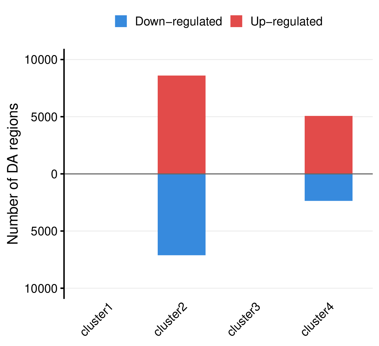
| group | n_rows_before | n_rows_after_nonzero | n_rows_after_mean | n_sig | n_up | n_down |
|---|---|---|---|---|---|---|
| cluster1 | 3860350 | 340850 | 340850 | 0 | 0 | 0 |
| cluster2 | 3860350 | 1201048 | 1201048 | 15709 | 8597 | 7112 |
| cluster3 | 3860350 | 341781 | 341781 | 0 | 0 | 0 |
| cluster4 | 3860350 | 528144 | 528144 | 7433 | 5070 | 2363 |
- Summary plot per comparison -
<comparison>/summary.pdf
- Mirror bar chart visualizing the number of differentially accessible regions per group, with up-regulated regions shown in red (above x-axis) and down-regulated regions in blue (below x-axis).
Example Usage
library(multiEpiCore)

# Test data
cm_root_path <- "count_matrix/"
cm_files <- c("C1_Count_Matrix_800.feather", "C2_Count_Matrix_800.feather", "T1_Count_Matrix_800.feather", "T2_Count_Matrix_800.feather")
cm_path <- file.path(cm_root_path, cm_files)

conditions <- c("C", "C", "T", "T")
sample_names <- c("C1", "C2", "T1", "T2")

out_dir <- "differential"

differential_regions(cm_path = cm_path, conditions = conditions, out_dir = out_dir, norm_level = "crf", min_support = 2, lfc_threshold = 0.5, p_threshold = 0.05, p_type = "fdr")
2. Differential Accessibility Heatmaps
The differential_heatmap() function generates
per-comparison, per-group heatmaps for all significant differential
regions produced by differential_regions(). It iterates
over the full result object returned by
differential_regions() and dispatches each comparison-group
combination to differential_heatmap_single(), which renders
a region × sample log2-CPM heatmap as a PDF file.
Log2-CPM values are read directly from the
_sig_log2_cpm.tsv output of
differential_regions(), which are derived from voom
transformation using globally estimated TMM normalization factors. No
additional transformation is applied.
When the underlying analysis used column clustering
(col_cluster_file_path), columns in the heatmap represent
individual sample:pair combinations within the cluster,
grouped and titled by sample. Without clustering, each column represents
one sample directly.
Parameters
| Parameter | Type | Default | Description | Example |
|---|---|---|---|---|
dr_result
|
nested list | — |
The return value of differential_regions(). A two-level
nested list structured as dr_result[[grp_name]][[cmp_tag]],
where the first level keys are cluster or pair names
(e.g. “cluster4”, “H3K27ac_peak1”) and the
second level keys are comparison tags (e.g. “T_vs_C”). Each
leaf is the file path to the corresponding _sig_counts.tsv.
|
dr_result <- differential_regions(…)
|
out_dir
|
character |
“./”
|
Output directory for heatmap PDFs. Created recursively if it does not
exist. One PDF is written per comparison-group combination, named
<cmp_tag>_<grp_name>.pdf.
|
“heatmaps”
|
show_colnames
|
logical |
FALSE
|
Whether to display individual column names on the heatmap. When
FALSE, only the sample-level column group titles are shown.
Set to TRUE to additionally show individual pair
identifiers within each sample group.
|
TRUE
|
col_width_mm
|
numeric |
40
|
Width per individual pair column in mm. Total heatmap width is computed
as n_pairs × col_width_mm + (n_samples − 1) × 8 mm, where
the second term accounts for the fixed 8 mm gap between sample groups.
In cluster mode (when col_cluster_file_path was supplied to
differential_regions()), each sample group contains
multiple pair columns; col_width_mm still refers to a
single pair column, so wider clusters automatically occupy
proportionally more space. In non-cluster mode each sample has exactly
one column, so col_width_mm equals the per-sample width
directly.
|
30
|
row_height_mm
|
numeric |
0.5
|
Height per region row in mm. Total heatmap body height is
n_sig_regions × row_height_mm mm, so the PDF scales
automatically with the number of significant regions. Note that values
below ~0.35 mm (one pixel at 72 dpi) will be visually indistinguishable;
for large region counts (>1000) a value of 0.13–0.5 mm produces dense
stripe patterns comparable to a fixed-height layout.
|
1.0
|
random_seed
|
integer |
42
|
Random seed passed to set.seed() before each raster
rendering call to ensure pixel-level reproducibility across runs.
|
123
|
Output Files
Output is organized by comparison tag (cmp_tag) read
from dr_result:
- Heatmap -
<comparison>/<cluster|pair>.pdf
- Rows: Significant genomic regions
- Columns: All CRF pairs across all samples
- Column blocks: Grouped by sample
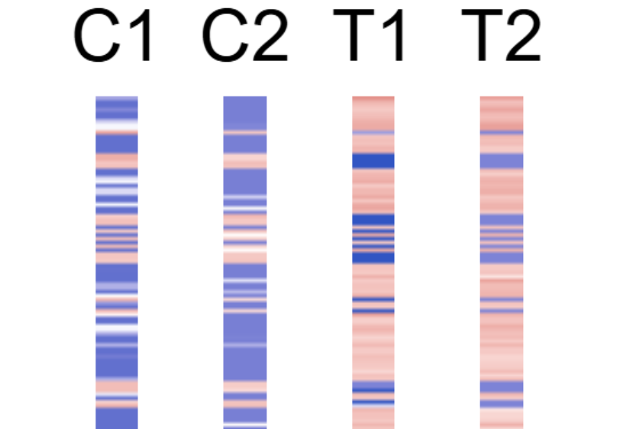
This figure shows differential analysis heatmap for cluster 4 in the test dataset.
Example Usage
library(multiEpiCore)

# Test data
dr_result <- list(
  H3K4me1 = list(
    T_vs_C = "differential/T_vs_C/H3K4me1_sig_log2_cpm.tsv"
  ),
  H3K27me3 = list(
    T_vs_C = "differential/T_vs_C/H3K27me3_sig_log2_cpm.tsv"
  ),
  H3K4me3 = list(
    T_vs_C = "differential/T_vs_C/H3K4me3_sig_log2_cpm.tsv"
  ),
  H3K9me3 = list(
    T_vs_C = "differential/T_vs_C/H3K9me3_sig_log2_cpm.tsv"
  )
)

differential_heatmap(
  dr_result = dr_result,
  out_dir   = "differential"
)
3. Differential Pathway Annotation
The differential_pathway_annotation() function performs
pathway enrichment analysis on the significant differential regions from
each comparison-group combination using GREAT (Genomic
Regions Enrichment of Annotations Tool). GREAT assigns genomic regions
to nearby genes via basal-plus-extension TSS domains, then tests for
over-representation of gene sets using a binomial test. Gene sets are
sourced from MSigDB via the
msigdbr package, and can be configured to use any available
collection such as Hallmark, Reactome, or GO terms.
Each comparison-group combination (e.g. T vs C within cluster 4) is tested independently. Results are written as per-comparison TSV tables and optionally visualised as a bubble plot that summarises enrichment patterns across all comparisons at a glance.
Parameters
| Parameter | Type | Default | Description | Example |
|---|---|---|---|---|
dr_result
|
nested list | — |
The return value of differential_regions(). A two-level
nested list structured as dr_result[[grp_name]][[cmp_tag]],
where each leaf is the file path to the corresponding
_sig_counts.tsv. Each comparison-group combination becomes
one GREAT query set.
|
dr_result <- differential_regions(…)
|
out_dir
|
character |
“./”
|
Output directory for enrichment TSV tables and the bubble plot PDF.
Created recursively if it does not exist. One TSV is written per query
set, named
pathway_annotation_<cmp_tag>_<grp_name>.tsv.
|
“pathway”
|
ref_genome
|
character |
“hg38”
|
Reference genome. Controls both the TSS source used by GREAT
(“hg38” → TxDb.Hsapiens.UCSC.hg38.knownGene,
“mm10” → TxDb.Mmusculus.UCSC.mm10.knownGene)
and the species passed to msigdbr(). Must be one of
“hg38” or “mm10”.
|
“mm10”
|
msigdb_collection
|
character |
“H”
|
MSigDB collection abbreviation. Common values: “H”
(Hallmark, 50 curated biological states), “C2” (curated
gene sets including KEGG and Reactome), “C5” (GO gene
sets). See msigdbr::msigdbr_collections() for the full
list.
|
“C2”
|
msigdb_subcollection
|
character or NULL |
NULL
|
MSigDB sub-collection abbreviation. Required when
msigdb_collection has subcollections. For example,
“CP:REACTOME” or “CP:KEGG_LEGACY” under
“C2”, and “GO:BP”, “GO:MF”, or “GO:CC” under “C5”. Leave
NULL for collections without subcollections such as
“H”.
|
“CP:REACTOME”
|
plot
|
logical |
TRUE
|
Whether to generate a bubble plot PDF
(pathway_annotation.pdf) summarising enrichment across all
query sets. Each row is a pathway ordered by best adjusted p-value
across query sets; bubble size encodes log2(1 +
fold_enrichment) and color encodes −log10(padj).
|
FALSE
|
Output Files
Output is organized by comparison tag (cmp_tag) read
from dr_result, with a pathway_annotation/
subdirectory created under each:
- Enrichment tables —
<cmp_tag>/pathway_annotation/pathway_annotation_<grp_name>.tsv
pathway: Pathway or gene set name, with collection-specific prefixes removed (e.g.HALLMARK_stripped for collection"H")hits_region: Number of input regions associated with at least one gene in the gene setfold: Fold enrichment of observed over expected region hitsp: Binomial test p-valuepadj: BH-adjusted p-value across all tested gene setshits_gene: Number of genes in the gene set that were hit by at least one input region
| pathway | hits_region | fold | p | padj | hits_gene |
|---|---|---|---|---|---|
| <chr> | <int> | <dbl> | <dbl> | <dbl> | <int> |
| ESTROGEN_RESPONSE_LATE | 244 | 1.78876440259542 | 0 | 0 | 93 |
| ESTROGEN_RESPONSE_EARLY | 274 | 1.64177634983608 | 9.10382880192628e-15 | 2.27595720048157e-13 | 108 |
| HEME_METABOLISM | 190 | 1.73776878897854 | 1.16373577441209e-12 | 1.93955962402015e-11 | 103 |
| P53_PATHWAY | 190 | 1.64117297423522 | 1.13204001728207e-10 | 1.41505002160258e-09 | 93 |
| XENOBIOTIC_METABOLISM | 150 | 1.52753944328334 | 5.99881082585796e-07 | 5.99881082585796e-06 | 74 |
| UV_RESPONSE_UP | 148 | 1.51216326635538 | 1.21354342041968e-06 | 1.01128618368307e-05 | 69 |
| TNFA_SIGNALING_VIA_NFKB | 233 | 1.36779498873411 | 2.32856113802082e-06 | 1.66325795572916e-05 | 103 |
| MYOGENESIS | 184 | 1.40053220922372 | 6.98954861699796e-06 | 4.34747783594079e-05 | 92 |
| ADIPOGENESIS | 158 | 1.43866050478738 | 7.82546010469343e-06 | 4.34747783594079e-05 | 77 |
| APOPTOSIS | 151 | 1.38058995740476 | 8.36612342312026e-05 | 0.000418306171156013 | 78 |
| … | … | ||||
This table shows pathway annotation result for cluster 4 in the test dataset.
- Bubble plot —
<cmp_tag>/pathway_annotation/pathway_annotation.pdf(whenplot = TRUE)
- Rows are pathways ordered by best adjusted p-value across all clusters/pairs.
- Columns are clusters/pairs.
- Bubble size encodes log2 fold enrichment and color encodes -log10(padj).
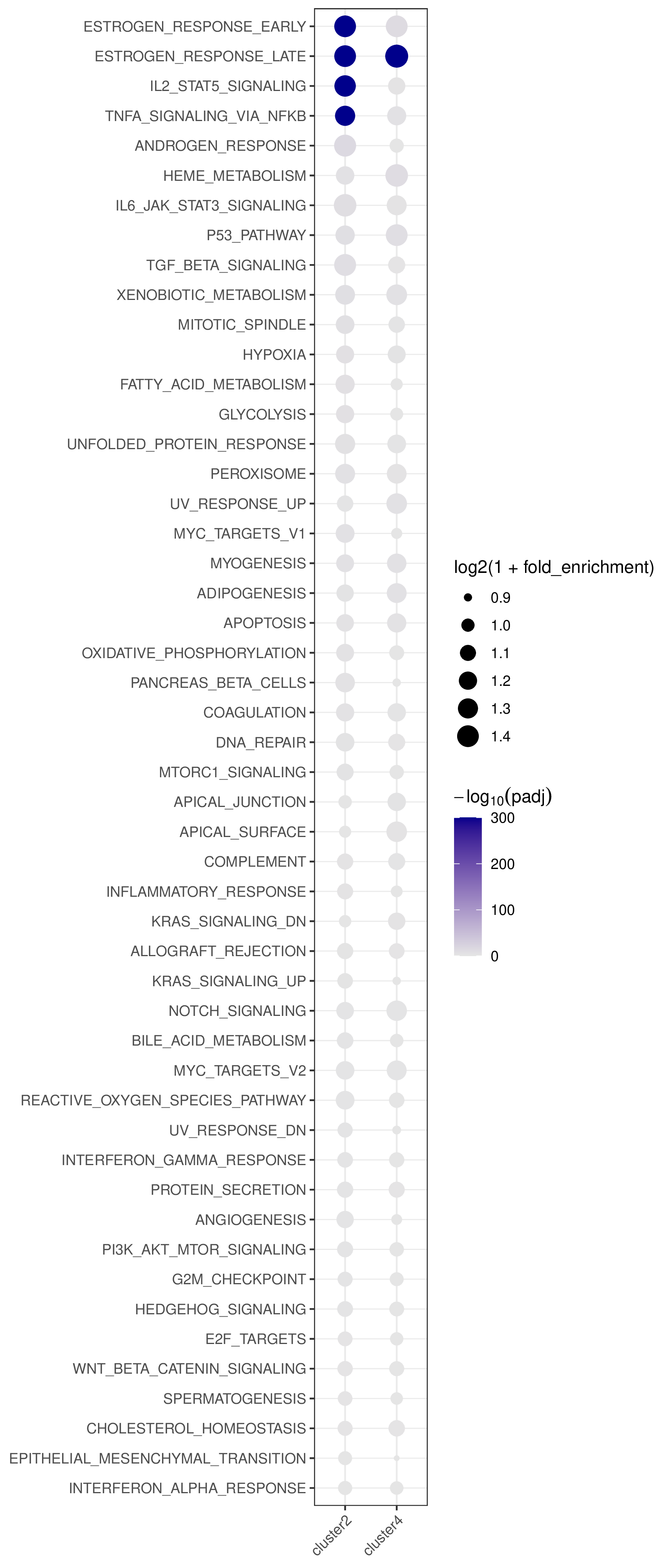
This figure shows pathway annotation result for cluster 4 in the test dataset.
Example Usage
library(multiEpiCore)

# Test data
dr_result <- list(
  H3K4me1 = list(
    T_vs_C = "differential/T_vs_C/H3K4me1_sig_log2_cpm.tsv"
  ),
  H3K27me3 = list(
    T_vs_C = "differential/T_vs_C/H3K27me3_sig_log2_cpm.tsv"
  ),
  H3K4me3 = list(
    T_vs_C = "differential/T_vs_C/H3K4me3_sig_log2_cpm.tsv"
  ),
  H3K9me3 = list(
    T_vs_C = "differential/T_vs_C/H3K9me3_sig_log2_cpm.tsv"
  )
)

differential_pathway_annotation(
  dr_result = dr_result,
  out_dir   = "differential/pathway_annotation"
)