Biclustering Analysis
Wrapper Function
The biclustering_wrapper() function runs the full
biclustering analysis workflow in one call. It optionally merges
multiple input matrices, applies transformations, performs highly
variable region filtering, runs biclustering on the filtered matrix, and
generates downstream annotation results including genomic distribution
summaries and TFBS enrichment. For users who prefer fine-grained control
over parameters, please refer to the detailed parameter settings
below.
Parameters
| Parameter | Type | Default | Description | Example |
|---|---|---|---|---|
cm_path
|
character / character vector | — |
Path to the input count matrix in .feather format, or a
vector of paths to multiple matrices. When a vector is provided (length
> 1), matrices are merged before downstream processing.
|
cm_path = c(“cm1.feather”, “cm2.feather”)
|
out_dir
|
character | — | Output directory for all generated files, including transformed matrices, cluster tables, and annotation results. |
out_dir = “./biclustering_out”
|
transformations
|
character vector |
c(“remove0”, “libnorm”, “log2p1”)
|
Vector specifying the transformation pipeline applied to the count matrix before biclustering. Steps are executed in order, and the behavior depends on the sequence you provide (see the table below for details). |
transformations = c(“remove0”, “libnorm”, “log2p1”,
“qnorm”)
|
filter_method
|
character |
“top_pct”
|
Method used to filter genomic regions prior to biclustering. One of
“top_pct”, “hvr”, or “none”. Use
“top_pct” (union of top-percentile regions across CRF
pairs) or “hvr” (highly variable regions) when the genome
was segmented into equal-sized bins (numeric regions), so
that low-information or uninformative bins can be removed. Use
“none” when the input matrix was built from user-provided
intervals (region file path), where additional filtering is typically
unnecessary.
|
filter_method = “hvr”
|
row_km
|
integer |
15
|
Number of k-means clusters for rows (genomic regions). |
row_km = 20
|
col_km
|
integer |
6
|
Number of k-means clusters for columns (CRF pairs). |
col_km = 4
|
apply_annotation
|
logical |
TRUE
|
Whether to perform downstream annotation on biclustered regions,
including genomic distribution summaries and TFBS enrichment.
Recommended for binned genomes (numeric regions). For
user-specified regions, set to FALSE if annotation is not
needed.
|
apply_annotation = TRUE
|
ref_genome
|
character |
“hg38”
|
Reference genome version used in annotation and control region
generation. Supported: “hg38”, “mm10”.
|
ref_genome = “mm10”
|
ref_source
|
character |
“knownGene”
|
Gene annotation source used in downstream analysis. Supported:
“knownGene” (UCSC knownGene via TxDb),
“GENCODE”.
|
ref_source = “GENCODE”
|
distributions
|
character vector |
c(“genic”,“ccre”)
|
Genomic feature distributions to summarize in the annotation step.
Options include: “genic”, “ccre”,
“cpg”, “repeat”.
|
distributions = c(“genic”,“repeat”)
|
plot
|
logical |
TRUE
|
Whether to generate diagnostic plots during filtering and biclustering
steps. This controls plotting behavior in detect_hvr() and
biclustering().
|
plot = FALSE
|
Example Usage
library(multiEpiCore)
# Test Data
cm_path <- c("count_matrix/C1_Count_Matrix_merged.feather",
             "count_matrix/C2_Count_Matrix_merged.feather")
biclustering_wrapper(
  cm_path = cm_path,
  out_dir = "bicluster",
  distributions = c("genic","ccre", "chromhmm", "repeat")
)
1. Merge Count Matrices
The merge_count_matrices() function merges multiple
count matrices (Feather files) into a single count matrix by aligning
genomic regions and combining counts across samples.
Parameters
| Parameter | Type | Default | Description |
|---|---|---|---|
cm_path
|
character vector | - |
A vector of feather file paths to be merged (.feather)
|
out_dir
|
character |
“./”
|
Output directory |
check_consistency
|
boolean |
TRUE
|
If TRUE, only keep rows (regions) and columns (targets)
that exist in all input files. If FALSE, merge all
rows and columns, filling missing values with 0.
|
Example Usage
library(multiEpiCore)
# Test Data
cm_path <- c(
  "count_matrix/C1_Count_Matrix_800.feather",
  "count_matrix/C2_Count_Matrix_800.feather"
)
merge_count_matrices(cm_path = cm_path, out_dir = out_dir)
2. Apply transformation
The apply_transformations() function performs a
sequential series of normalization and transformation steps on a count
matrix and outputs the processed result.
Parameters
| Parameter | Type | Default | Description |
|---|---|---|---|
cm_path
|
character | - |
Path to the input count matrix (.feather). The input file must be a
valid .feather file containing a positional column
(pos) or any first column that uniquely identifies genomic
intervals. All remaining columns must be numeric.
|
out_dir
|
character |
“./”
|
Output directory |
transformations
|
character vector |
c(“remove0”, “libnorm”, “log2p1”)
|
Vector specifying the transformation pipeline. Steps are executed in order, and the behavior depends on the sequence you provide (see the table below for details). |
save_each_step
|
logical |
FALSE
|
If TRUE, writes a .feather file after each
step, allowing inspection of intermediate matrices.
|
The order of operations in transformations directly
determines the output. Below is the full list of supported steps:
| Transformation | Description |
|---|---|
remove0 |
Remove regions where all targets have zero counts |
libnorm |
Library size normalization (CPM, counts per million) |
log2p1 |
Log2 transformation: log2(x + 1) |
sqrt |
Square root transformation |
minmaxnorm |
Scale values to [0, 1] range |
qnorm |
Quantile normalization across targets |
zscore |
Z-score standardization across regions |
Output Files
After processing all selected transformations, a final Feather file named:
<original_name>_transformed.featherIf set save_each_step = TRUE, the output path will
be:
out_dir/
├── [count_matrix_prefix]_transformed.feather
├── [count_matrix_prefix]_remove0.feather
├── [count_matrix_prefix]_remove0_libnorm.feather
├── [count_matrix_prefix]_remove0_libnorm_log2p1.feather
└── [count_matrix_prefix]_remove0_libnorm_log2p1_qnorm.feather
Example Usage
library(multiEpiCore)
# Test Data
apply_transformations(
  cm_path = "Count_Matrix_merged.feather",
  transformations = c("remove0", "libnorm", "log2p1", "qnorm"),
  out_dir  = "bicluster",
  save_each_step  = FALSE
)
3. Region Filtering
Constructing the count matrix by tiling the genome into fixed-size bins yields several million candidate regions, which imposes substantial computational burden on downstream clustering. Moreover, the majority of these bins (~99%) typically have zero read counts across all CRF target pairs and carry no biologically meaningful signal. A filtering step is therefore required to reduce the count matrix to an informative subset of regions prior to biclustering. Two complementary filtering strategies are provided:
Top-Percentile (filter_top_pct) |
HVR (detect_hvr) |
|
|---|---|---|
| Selection criterion | Fixed per-pair quantile threshold on transformed values | Bin-level deviation from a fitted mean–variance trend |
| Limitation | Threshold is not adaptive to signal quality: for pairs with weak
true biological variability, a fixed top_pct is still
enforced, which can admit noise-driven bins; selection also does not
account for mean–variance structure and may instead reflect differences
in coverage depth across pairs |
Selected regions may be disproportionately dominated by a subset of CRF pairs with globally high variance, under-representing pairs with more modest but still genuine signal |
| When to use | To guarantee a fixed, consistent proportion of bins selected from each pair, regardless of that pair’s overall variance | To retain regions with unusually large variability relative to their expected mean–variance relationship |
3A. Top Percentile Filtering
The filter_top_pct() function selects highly ranked
genomic regions based on their transformed signal value within each CRF
pair, without modeling the mean–variance relationship.
What this function does:
(Per-pair thresholding) For each CRF pair column, computes the value at the
(1 - top_pct)quantile of that pair’s transformed signal, defining a pair-specific cutoff.(Union selection) Retains any bin that meets or exceeds its own pair’s threshold in at least one pair, taking the union of top-ranked bins across all pairs rather than intersecting them.
(Output) Writes the transformed count matrix, subsetted to the union of selected bins, to a feather file in the same layout as
filter_hvr()’s output, making it a drop-in alternative for downstream biclustering. An optional diagnostic plot shows the per-pair threshold value and number of bins selected.
Parameters
| Parameter | Type | Default | Description | Example |
|---|---|---|---|---|
transformed_cm_path
|
character | — |
Path to the transformed count matrix file in .feather
format. The file must contain a pos column.
|
transformed_cm_path = “data_transformed.feather”
|
out_dir
|
character |
“./”
|
Output directory path for the filtered matrix (and diagnostic plot, if requested). |
out_dir = “./filtered_results”
|
top_pct
|
numeric |
0.001
|
Fraction (range: 0–1, exclusive) defining the “top” cutoff applied
independently to each CRF pair column. For a given pair, only
bins at or above that pair’s (1 - top_pct) quantile of
transformed values are selected. The final output is the
union of bins selected across all pairs, so the total
number of retained bins is not a fixed proportion of the genome and can
exceed top_pct in practice.
|
top_pct = 0.01
|
plot
|
logical |
FALSE
|
Whether to generate a diagnostic plot showing, per pair, the
top_pct threshold value and the number of bins selected.
|
plot = TRUE
|
Output Files
The function generates the following output files in the specified
out_dir (default: “./”):
- Filtered Count Matrix File -
Filtered_TopPct_<top_pct>.feather- Feather format dataframe containing the transformed count matrix subsetted to the union of top-ranked bins
- Same column layout as the input transformed count matrix (and as
filter_hvr()’s output), making it a drop-in replacement wherever afiltered_cm_pathis expected downstream
| H3K27ac-H3K4me3 | H3K27me3-H3K27me3 | H3K27me3-H3K4me1 | H3K27me3-H3K4me3 | |
|---|---|---|---|---|
| chr1_924754_925901 | 0.0000000 | 1.2513753 | 0.6080126 | 1.7774121 |
| chr1_960217_961971 | 0.0000000 | 0.8588573 | 0.6080126 | 0.5887534 |
| chr1_1304439_1306480 | 0.9310723 | 0.9001684 | 1.3631568 | 2.0490081 |
| chr1_2231096_2232510 | 6.2389879 | 2.1113949 | 3.0607326 | 5.3591691 |
| chr1_3771354_3772564 | 4.8683023 | 0.0000000 | 1.8563049 | 4.3285168 |
| … | … | … | … | … |
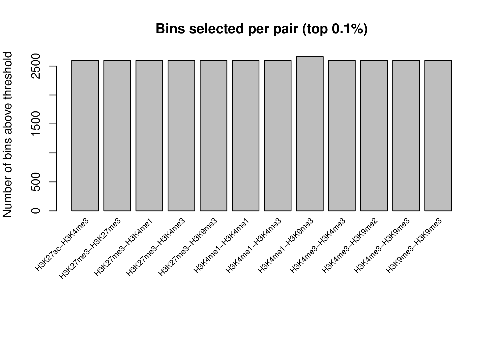
- Diagnostic Plot (optional, when
plot = TRUE) -filter_top_pct_diagnostic.pdf- Bar plot showing, for each CRF pair, the number of bins selected
above that pair’s
top_pctthreshold - Pair labels are rotated 45° along the x-axis for readability
- Useful for confirming that no single pair is disproportionately over- or under-represented in the final union
- Bar plot showing, for each CRF pair, the number of bins selected
above that pair’s
3B. Highly Variable Regions (HVR)
The detect_hvr() function identifies highly variable
genomic regions by modeling the mean–variance relationship of
transformed count data and selecting regions whose variability exceeds
technical expectations.
What this function does:
(Model mean–variance relationship) Fits a regression model in log2 space to characterize the global relationship between mean signal intensity and variance across all genomic regions, capturing the baseline mean–variance trend expected under technical variation.
(Quantify overdispersion) For each region, estimates the expected variance given its mean signal level from the fitted model, then normalizes the observed signal by this expectation to compute a hypervariance metric — the region’s deviation from the mean–variance trend after accounting for mean-dependent variance effects. Regions with hypervariance > 1 exhibit variability exceeding technical expectation, consistent with biological heterogeneity rather than noise.
(Stratified selection) Divides the log2(mean) expression range into equal-sized bins and selects the top hypervariant regions within each bin, ensuring balanced representation across low, medium, and high expression levels rather than favoring highly expressed regions by default.
(Expression threshold) Applies a percentile-based cutoff to exclude lowly expressed regions, which are disproportionately susceptible to noise-driven hypervariance estimates.
(Output) Writes the filtered, transformed count matrix to a feather file for downstream biclustering, along with region-level statistics (observed mean/variance, expected variance, normalized values, hypervariance) for quality control. Optional diagnostic plots visualize the fitted mean–variance trend with selected regions highlighted, and the hypervariance distribution across expression bins with selection boundaries, confirming balanced sampling across expression levels.
Parameters
| Parameter | Type | Default | Description | Example |
|---|---|---|---|---|
transformed_cm_path
|
character | — |
Path to the transformed count matrix file in .feather
format. The file must contain a pos column.
|
transformed_cm_path = “data_transformed.feather”
|
out_dir
|
character |
“./”
|
Output directory path for all generated results. |
out_dir = “./hvr_results”
|
keep_percent
|
numeric |
0.01
|
Fraction of total regions to retain (range: 0–1). Selected regions are distributed equally across all bins. |
keep_percent = 0.05
|
log2mean_quantile_thres
|
numeric |
0.99
|
Quantile threshold (range: 0–1) applied to log2(mean) expression. Only regions above this threshold are retained in the final selection. |
log2mean_quantile_thres = 0.95
|
plot
|
logical |
FALSE
|
Whether to generate diagnostic plots for both MAV screening and feature selection steps. |
plot = TRUE
|
Region filtering behavior:
- Regions with
hypervar ≤ 1are automatically excluded as they represent regions with expected or reduced variance (not informative for downstream analysis) - The stratified binning ensures balanced selection across expression levels, preventing bias toward highly expressed regions
- The final
log2mean_quantile_thresthreshold removes lowly expressed regions that may be dominated by technical noise
- Regions with
Parameter tuning recommendations: If your analysis yields too few selected regions, this typically occurs when you’re analyzing a targeted genomic subset (e.g., promoter regions, CpG islands, specific gene loci) rather than genome-wide bins. The combination of default
keep_percent = 0.01(1%) andlog2mean_quantile_thres = 0.99(99th percentile) is too stringen.Scenario keep_percentlog2mean_quantile_thresExpected output Genome-wide bins (default) 0.01 (1%) 0.99 (99th) ~1,000-5,000 regions Targeted regions (promoters, peaks) 0.05-0.10 (5-10%) 0.90-0.95 (90-95th) ~2,000-10,000 regions Very sparse data 0.10-0.20 (10-20%) 0.85-0.90 (85-90th) ~5,000-20,000 regions Large datasets (>100K input regions) Reduce n_binsto 50Keep defaults Faster computation
Output Files
The function generates the following output files in the specified
out_dir (default: “./”):
- Filtered Count Matrix -
<input_name>_filtered_regions.feather- Feather format file containing count data for filtered regions
- First column “pos” contains region identifiers
- Subsequent columns contain count values for each target
- Only includes regions passing all selection criteria:
- Hypervariance > 1 (overdispersed)
- Top hypervariant features within each log2(mean) bin
- log2(mean) above the specified quantile threshold
- Dimensions: n_selected_regions × (n_targets + 1)
| H3K27me3-H3K4me3 | H3K27me3-H3K9me3 | H3K4me1-H3K4me1 | H3K4me1-H3K4me3 | |
|---|---|---|---|---|
| chr1_924754_925901 | 4.328517 | 0.000000 | 2.055202 | 5.196457 |
| chr1_960217_961971 | 2.721607 | 0.170777 | 0.000000 | 2.796186 |
| chr1_1304439_1306480 | 5.184029 | 2.486189 | 4.232496 | 5.770927 |
| chr1_2231096_2232510 | 5.537428 | 2.355185 | 4.091192 | 6.427042 |
| chr1_3771354_3772564 | 4.544285 | 1.340344 | 2.947109 | 5.426958 |
| … | … | … | … | … |
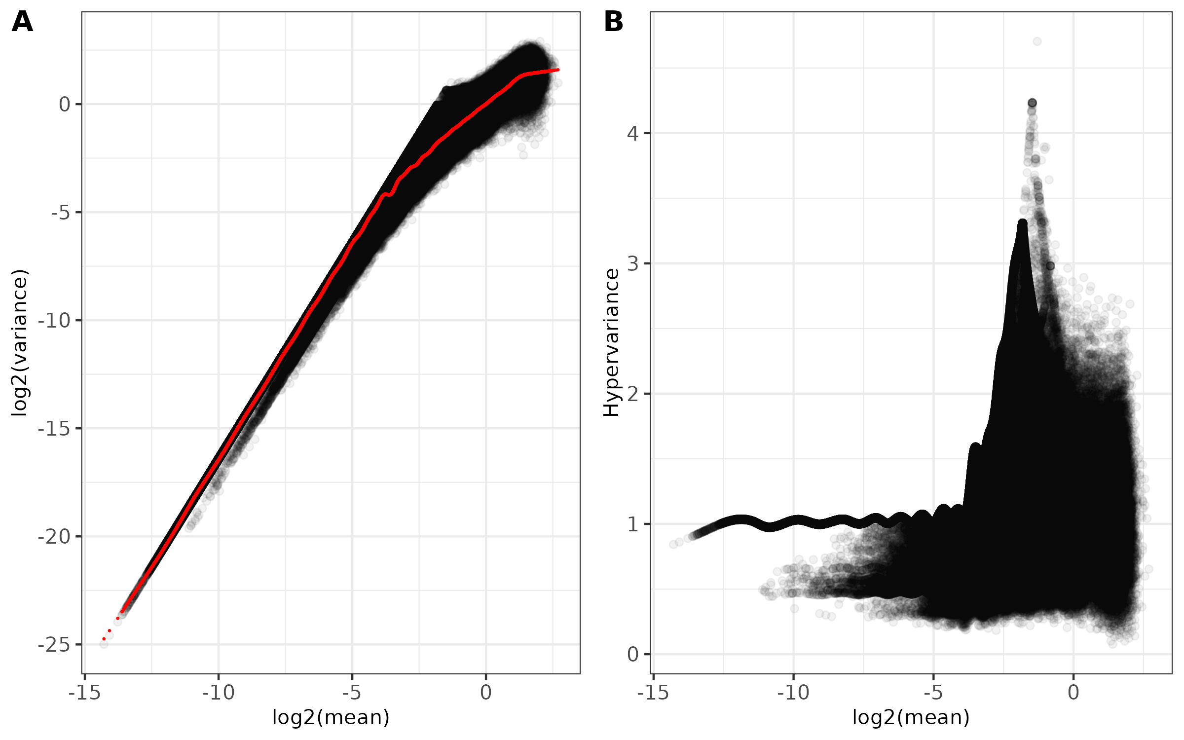
- Main diagnostic plots -
<input_name>_mean_variance.png(ifplot = TRUE)- Combined two-panel figure showing:
- Panel A: Log2(mean) vs Log2(variance) with fitted trend line in red
- Panel B: Log2(mean) vs Hypervariance
- Points shown with transparency to visualize density
- Theme: black and white with customizable font size
- Saved as PNG format
- Combined two-panel figure showing:
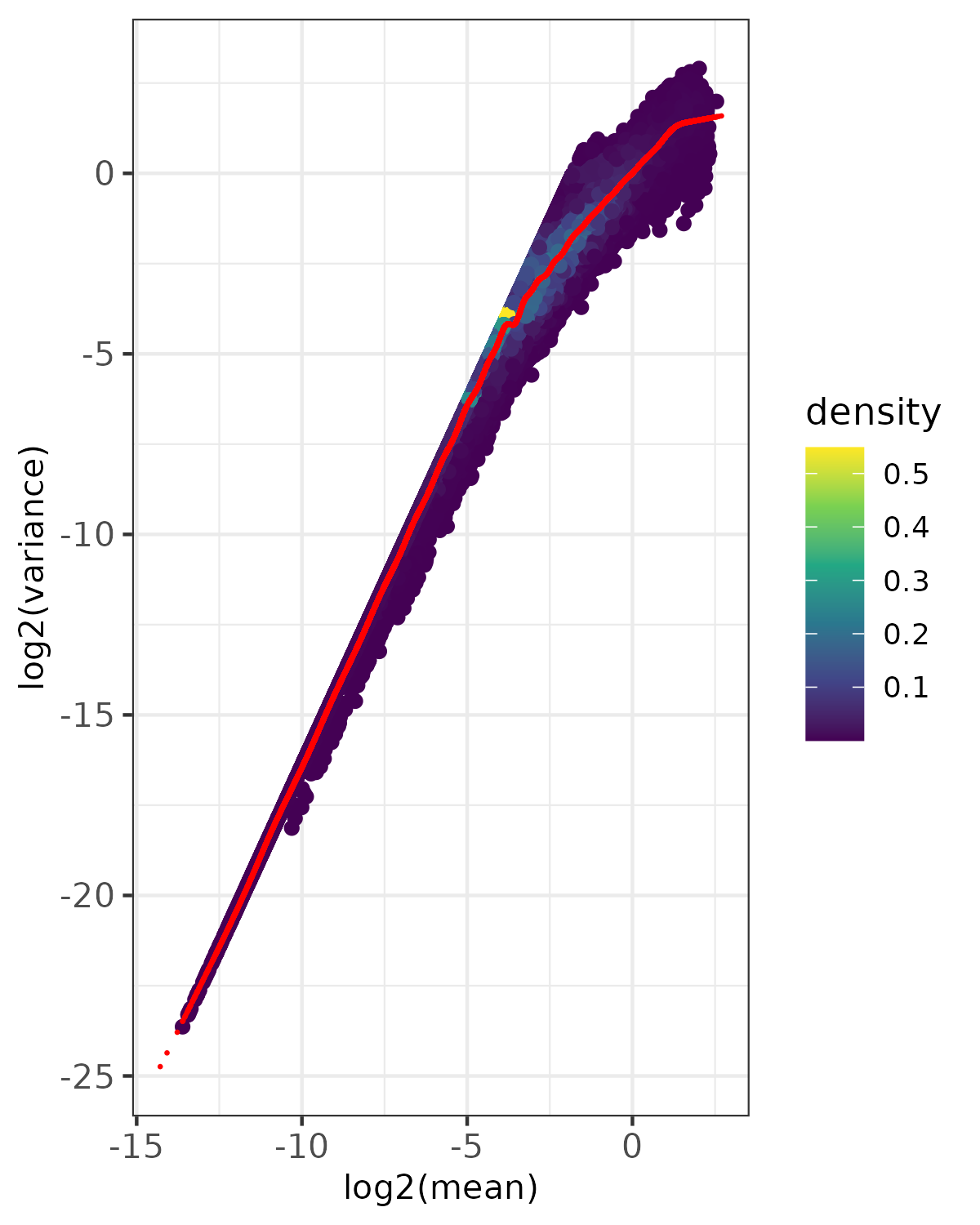
- Density plot -
<input_name>_fit_density.png(ifplot = TRUE)- Point density visualization of mean-variance relationship
- Uses viridis color scale to show point density
- Red points show expected variance from fitted model
- Based on randomly sampled subset of data (controlled by
nrow_sample_perandseed) - Useful for visualizing patterns in large datasets
- Saved as PNG format
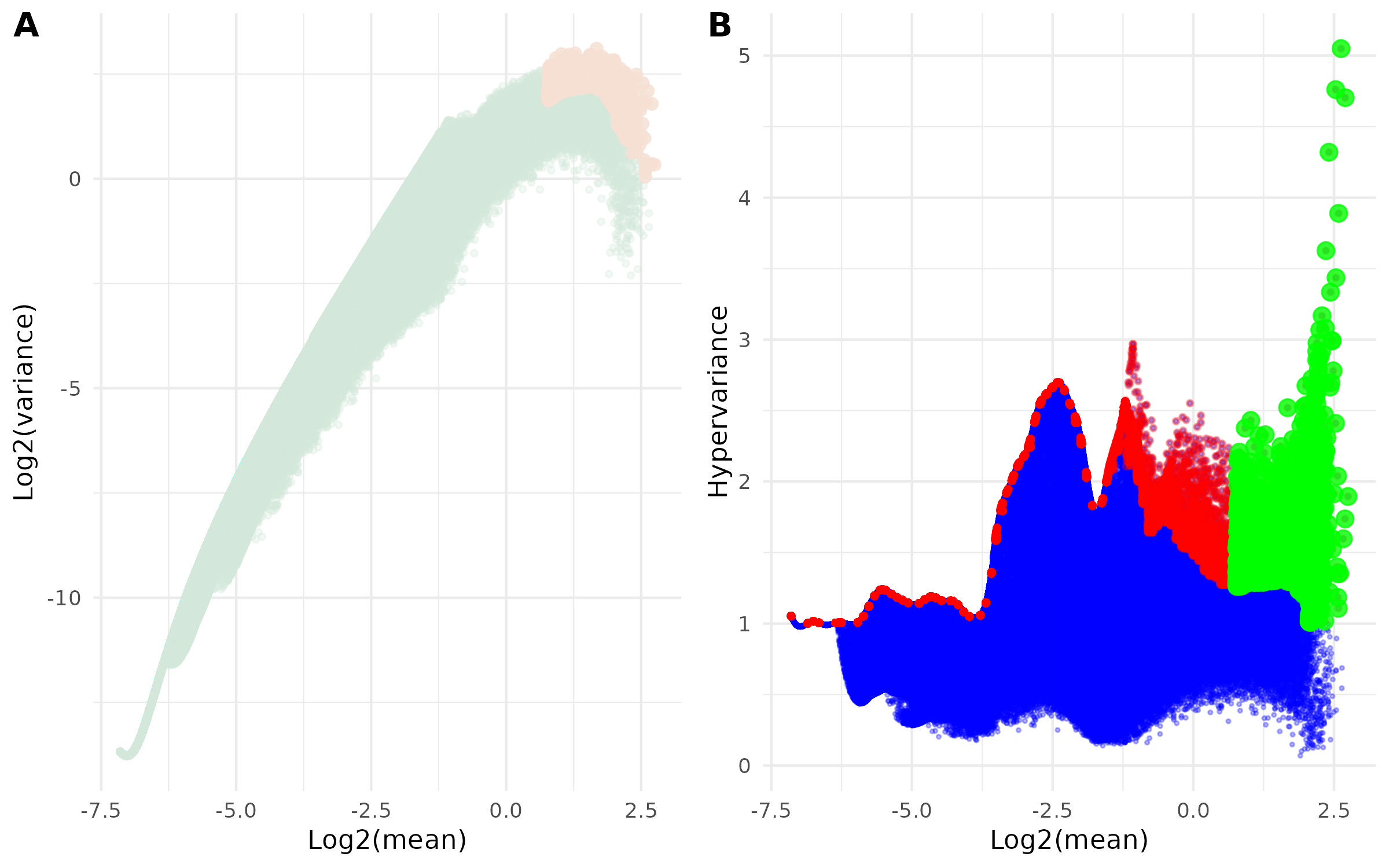
- Diagnostic Plots -
<input_name>_filtered_regions.png(ifplot = TRUE)
This combined figure contains two complementary visualizations of the selection process:
- Panel A: Mean-Variance Relationship
- Scatter plot of log2(mean) vs log2(variance)
- Shows how selected regions relate to overall mean-variance distribution
- Highlights selected regions:
- Light Green points: All regions
- Light Orange points: Final selected highly-variable regions
- Panel B: Hypervariance vs Expression
- Scatter plot of log2(mean) vs hypervariance
- Visualizes the selection process across expression levels
- Three layers of points:
- Blue points: All regions from hypervar summary
- Red points: Regions selected from binned filtering
- Green points: Final selected highly-variable regions after quantile filtering
Example Usage
library(multiEpiCore)
# Test Data
path <- "bicluster/Count_Matrix_merged_transformed.feather"
detect_hvr(transformed_cm_path = path, out_dir = "./count_matrix/", plot = TRUE)
4. Combinatory Landscape of Co-localized CRF Pairs
4A. Kmeans-based Biclustering and Heatmap Generation
The biclustering() function performs bidirectional
k-means clustering on genomic count matrices and generates cluster
assignment files along with publication-ready heatmap
visualizations.
What this function does:
(Consensus k-means clustering) Applies k-means clustering independently to rows (genomic regions) and columns (CRF pairs). For robustness, consensus clustering aggregates results from multiple k-means runs (controlled by
row_repeatsandcol_repeatsin the underlying algorithm) to identify stable cluster assignments.(Hierarchical cluster ordering) After initial k-means assignment, clusters are reordered hierarchically to optimize visual interpretation in heatmaps. For each dimension (rows/columns), cluster centroids (mean profiles) are calculated and hierarchically clustered using specified distance metrics and linkage methods. The resulting dendrogram is reordered by centroid weights to place similar clusters adjacent to each other.
(Within-cluster feature ordering) Within each cluster, individual features are reordered using hierarchical clustering to reveal internal structure and gradual transitions between expression patterns. This two-level organization (between-cluster + within-cluster) ensures both global pattern recognition and local detail preservation.
(Integrated heatmap generation) Automatically creates publication-ready heatmaps with the clustered and ordered matrix, using the generated cluster assignment files to add annotation tracks. Heatmap aesthetics (color ranges, font sizes, column name display) are fully customizable.
Parameters
| Parameter | Type | Default | Description | Example |
|---|---|---|---|---|
cm_path
|
character | — |
Path to the count matrix file in .feather format. The file
must contain a pos column, where rows represent genomic
positions and columns represent targets.
|
cm_path = “normalized_counts.feather”
|
row_km
|
integer | — | Number of k-means clusters applied to rows (genomic regions). |
row_km = 15
|
col_km
|
integer | — | Number of k-means clusters applied to columns (CRF pairs). |
col_km = 16
|
out_dir
|
character | — | Output directory used to save cluster assignment files and heatmap visualizations. |
out_dir = “./clustering_results”
|
seed
|
integer |
123
|
Random seed used to ensure reproducible k-means clustering results. |
seed = 42
|
plot
|
logical |
TRUE
|
Whether to generate and save the heatmap visualization. |
plot = FALSE
|
show_column_names
|
logical |
FALSE
|
Whether to display column names at the bottom of the heatmap. |
show_column_names = TRUE
|
lower_range
|
numeric |
NULL
|
Lower bound of the heatmap color scale. If NULL, the
minimum value from the data is used.
|
lower_range = 0
|
upper_range
|
numeric |
NULL
|
Upper bound of the heatmap color scale. If NULL, the
maximum value from the data is used.
|
upper_range = 10
|
row_title_fontsize
|
numeric |
NULL
|
Font size for row cluster titles (e.g. A, B, C). |
row_title_fontsize = 40
|
col_title_fontsize
|
numeric |
NULL
|
Font size for column cluster titles (e.g. 1, 2, 3). |
col_title_fontsize = 22
|
legend_title_fontsize
|
numeric |
NULL
|
Font size used for the heatmap legend title. |
legend_title_fontsize = 40
|
legend_label_fontsize
|
numeric |
NULL
|
Font size used for legend tick labels. |
legend_label_fontsize = 30
|
Input requirements:
- Count matrix must be in .feather format
- First column must be named “pos” containing region identifiers
- Matrix must contain numeric values only
Reproducibility: Always set
seedparameter for reproducible results, as k-means involves random initialization.Color scale interpretation:
- Default: Auto-scales to data range
- Custom: Use
lower_rangeandupper_rangefor consistent scales across analyses - Blue = Low signal, White = Medium, Red = High signal
Output Files
The function generates the following output files in the specified
out_dir:
- Row cluster assignments -
row_table.tsv- Tab-separated file with row cluster assignments
- Two columns:
region: Genomic region identifier (e.g., “chr1_1000_2000”)cluster: Cluster label as letter (A, B, C, D, etc.)
- Sorted by cluster label for easy inspection
- Rows within each cluster are ordered by hierarchical clustering
- Used for annotating genomic regions by cluster membership
- Column cluster assignments -
col_table.tsv- Tab-separated file with column (target) cluster assignments
- Two columns:
pair: CRF pair identifier (e.g., “YY1-cJun”)cluster: Cluster label as number (1, 2, 3, etc.)
- Sorted by cluster label
- Columns within each cluster are ordered by hierarchical clustering
- Used for grouping targets by similarity
| pair | cluster | |
|---|---|---|
| <chr> | <dbl> | |
| 1 | H3K9me3-H3K9me3 | 1 |
| 2 | H3K27me3-H3K4me1 | 2 |
| 3 | H3K27me3-H3K27me3 | 2 |
| 4 | H3K27me3-H3K9me3 | 2 |
| 5 | H3K4me1-H3K4me1 | 3 |
| 6 | H3K4me1-H3K9me3 | 3 |
| 7 | H3K27ac-H3K4me3 | 4 |
| 8 | H3K4me1-H3K4me3 | 4 |
| 9 | H3K4me3-H3K4me3 | 4 |
| 10 | H3K4me3-H3K9me3 | 4 |
| 11 | H3K27me3-H3K4me3 | 4 |
| 12 | H3K4me3-H3K9me2 | 4 |
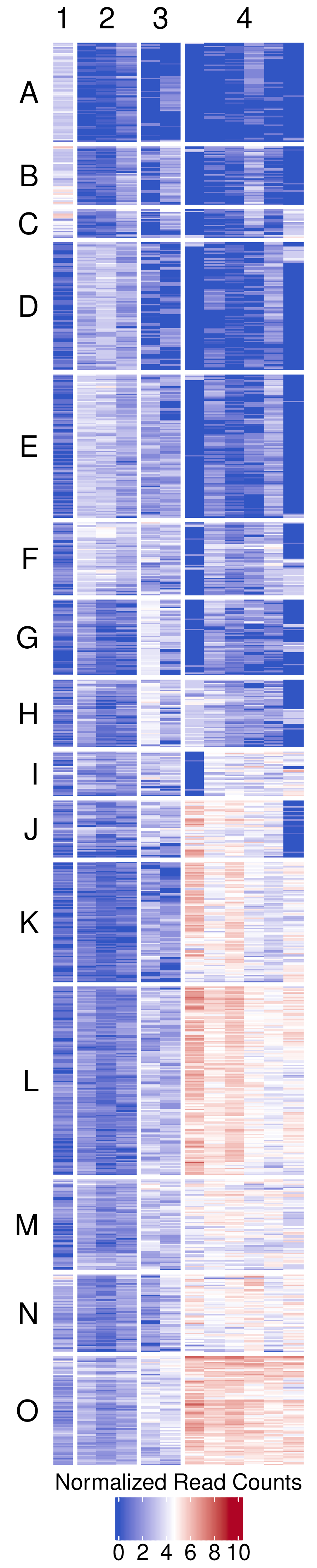
- Clustered heatmap -
figures/biclustering_heatmap.pdf- Publication-ready heatmap in PDF format
- Features:
- Rows organized by k-means clusters (labeled A, B, C, etc.)
- Columns organized by k-means clusters (labeled 1, 2, 3, etc.)
- Color scale: Blue (low) → White (middle) → Red (high)
- Horizontal legend positioned at bottom
- White gaps between clusters for visual separation (3mm)
- Customizable font sizes for titles and labels
- Transparent background for publication flexibility
- Dimensions automatically calculated based on matrix size
Example Usage
library(multiEpiCore)

# General Usage
cm_path <- "Count_Matrix_merged_transformed_mav_screen_filtered_regions.feather"
out_dir <- "."
biclustering(cm_path = cm_path, row_km = 15, col_km = 16, out_dir = out_dir)

# Test Data
cm_path <- "bicluster/Count_Matrix_merged_transformed_filtered_regions.feather"
out_dir <- "bicluster"
biclustering(cm_path = cm_path, row_km = 15, col_km = 4, out_dir = out_dir)
4B. (Optional) Add Non-Informative Regions Back to Clusters
The add_regions_back_to_cluster() function assigns
cluster labels to genomic regions that were excluded from the highly
variable set by correlating them with existing cluster signatures.
What this function does:
This function recovers regions that were filtered out during
highly-variability selection and assigns them to the row clusters
generated by the biclustering() function.
(Filter non-highly-variable regions) Starting with the original count matrix, the function identifies non-highly-variable regions (those excluded from clustering) and filters them based on a minimum non-zero count threshold at the raw count level. Specifically, regions must have non-zero counts in more than a specified number of targets (controlled by
cutoff_non_zero) to be considered for cluster assignment.(Correlation-based cluster assignment) For each row cluster from biclustering, the function calculates a signature profile by averaging the transformed expression values of highly variable regions assigned to that cluster. Non-highly-variable regions are then correlated against these cluster signatures using their transformed values. Regions with maximum correlation values exceeding the specified quantile threshold (controlled by
quantile_threshold) are assigned to their best-matching cluster.(Priority-based label assignment) The final output combines all regions into a priority-based classification:
- Original cluster assignments from biclustering (highest priority)
- Correlation-based assignments for high-correlation regions
- CRF_specific for low-correlation candidates that passed the non-zero filter
- Background for all remaining regions with non-zero counts
Parameters
| Parameter | Type | Default | Description | Example |
|---|---|---|---|---|
orig_cm_path
|
character | — |
Path to a .feather file containing the original count
matrix generated by build_count_matrix. The matrix includes
all regions in untransformed form, with pos as the first
column.
|
orig_cm_path = “count_matrix.feather”
|
transformed_cm_path
|
character | — |
Path to a .feather file containing transformed count data
(e.g. log-normalized or scaled) used for correlation analysis.
|
transformed_cm_path = “qnorm_counts.feather”
|
filtered_cm_path
|
character | — |
Path to a .feather file containing informative or
significant regions used in the original clustering analysis.
|
filtered_cm_path = “informative_regions.feather”
|
row_cluster_path
|
character | — |
Path to a TSV file defining cluster assignments for informative regions.
The file must include region and cluster
columns.
|
row_cluster_path = “row_table.tsv”
|
out_dir
|
character | — | Output directory used to save result tables and optional diagnostic plots. |
out_dir = “./results”
|
cutoff_non_zero
|
integer |
10
|
Minimum number of non-zero targets required per region. Regions with more than this number of non-zero values are retained. |
cutoff_non_zero = 15
|
quantile_threshold
|
numeric |
0.75
|
Quantile threshold (range: 0–1) for filtering high-correlation regions. Only regions above this quantile are assigned cluster labels. |
quantile_threshold = 0.80
|
plot
|
logical |
FALSE
|
Whether to generate and save a histogram of the correlation distribution. |
plot = TRUE
|
Input file requirements:
- All feather files must have ‘pos’ column as first column
cluster_pathTSV must have ‘region’ and ‘cluster’ columns
Non-zero filtering: The
cutoff_non_zero = 10means regions must have MORE than 10 non-zero targets (not equal to 10).Quantile threshold interpretation:
quantile_threshold = 0.75means only regions with correlation in the top 25% receive cluster assignments.
Output Files
The function generates the following output files in
out_dir:
- Complete region-cluster table -
row_table_all.tsv- Comprehensive table containing all genomic regions with assigned labels
- Two columns:
region: Genomic region identifier (chromosome coordinates)cluster: Assigned cluster label or category
- Label priority hierarchy (highest to lowest):
- Original cluster assignments: From
row_cluster_path(informative region clusters) - Correlation-based assignments: High-correlation regions matched to cluster signatures
- CRF_specific: Regions passing non-zero filter but below correlation threshold
- Background: All other regions with non-zero counts
- Original cluster assignments: From
- Tab-delimited format (.tsv)
- Includes all non-zero regions from the genome
region cluster chr1_9601_10400 J chr1_10401_11200 CRF_specific chr1_12801_13600 Background chr1_14401_15200 Background chr1_15201_16000 Background chr1_16001_16800 Background - Filtered region-cluster table -
row_table_clean.tsv- Contains only cluster-assigned regions (excludes “Background” and “CRF_specific” labels)
- Same two-column format as complete table
- Tab-delimited format (.tsv)
- Useful for downstream analyses focusing on clustered regions only
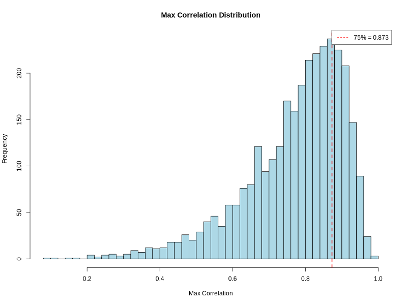
- Correlation distribution histogram -
correlation_histogram.png(ifplot = TRUE)- PNG format visualization showing distribution of maximum correlation values
- X-axis: Maximum correlation between regions and cluster signatures
- Y-axis: Frequency of regions
- Red dashed line: Quantile threshold for filtering
- Legend: Shows quantile threshold value
- Resolution: 800 × 600 pixels
- Helps visualize correlation quality and threshold selection
- Color scheme: Light blue bars with black borders
Example Usage
library(multiEpiCore)

# Test Data
orig_cm_path <- "count_matrix/Count_Matrix_merged.feather"
transformed_cm_path <- "bicluster/Count_Matrix_merged_transformed.feather"
filtered_cm_path <- "bicluster/Count_Matrix_merged_transformed_filtered_regions.feather"
row_cluster_path <- "bicluster/row_table.tsv"
out_dir <- "add_regions_results"

add_regions_back_to_cluster(
  orig_cm_path = orig_cm_path,
  transformed_cm_path = transformed_cm_path,
  filtered_cm_path = filtered_cm_path,
  row_cluster_path = row_cluster_path,
  out_dir = out_dir,
  cutoff_non_zero = 10,
  quantile_threshold = 0.75,
  plot = TRUE
)
4C. (Optional) Apply Pre-Computed Clusters to Generate Heatmaps
After adding non-highly-variable regions back to clusters, the
biclustering_heatmap() function can be used to generate
heatmaps using the expanded cluster assignments (typically from
row_table_clean.tsv). This function creates
publication-ready visualizations without re-running the clustering
algorithm. Note that this function is also called internally by the
biclustering() function to generate the initial heatmap
after performing bidirectional k-means clustering.
What this function does:
(Load and validate cluster assignments) Reads row and column cluster assignment files and validates that regions in the cluster files match those present in the input count matrix. Typically uses the clean cluster assignments (
row_table_clean.tsv) that exclude “Background” and “CRF_specific” labels.(Order matrix by clusters) Reorders the count matrix rows and columns according to cluster assignments, ensuring regions within the same cluster are grouped together for visualization.
(Configure color scaling) Sets up a diverging color scheme (blue → white → red) with customizable value ranges. If ranges are not specified, automatically determines appropriate bounds from the data.
(Calculate optimal dimensions) Automatically computes cell sizes and heatmap dimensions based on the number of clusters and their sizes, ensuring cluster labels are readable and properly positioned. Adjusts legend font sizes to fit within the available space.
(Generate publication-ready heatmap) Creates a PDF heatmap with:
- Rows split by cluster assignments (labeled A, B, C, …)
- Columns split by cluster assignments (labeled 1, 2, 3, …)
- White gaps between clusters for visual separation
- Horizontal legend at bottom showing color scale
- Transparent background for publication flexibility
- High-resolution rasterized cells for efficient rendering
Parameters
| Parameter | Type | Default | Description | Example |
|---|---|---|---|---|
mat
|
matrix | — | Count matrix with genomic regions as rows and targets as columns. The matrix must contain row names (region IDs) and column names (target IDs). |
mat = as.matrix(count_data)
|
row_cluster_file_path
|
character | — |
Path to a TSV file defining row cluster assignments. The file must
contain region and cluster columns. Typically
uses row_table_clean.tsv generated by
add_regions_back_to_cluster().
|
row_cluster_file_path = “row_table_clean.tsv”
|
col_cluster_file_path
|
character | — |
Path to a TSV file defining column cluster assignments. The file must
contain pair and cluster columns.
|
col_cluster_file_path = “col_table.tsv”
|
out_dir
|
character |
“./”
|
Output directory used to save the generated heatmap. |
out_dir = “./heatmaps”
|
show_column_names
|
logical |
FALSE
|
Whether to display target names along the column axis of the heatmap. |
show_column_names = TRUE
|
lower_range
|
numeric |
NULL
|
Lower bound for the heatmap color scale. If NULL, the
minimum value in the matrix is used.
|
lower_range = 0
|
upper_range
|
numeric |
NULL
|
Upper bound for the heatmap color scale. If NULL, the
maximum value in the matrix is used.
|
upper_range = 4.5
|
row_title_fontsize
|
numeric |
NULL
|
Font size for row cluster titles (e.g. A, B, C). If NULL, a
default size of 20 is used.
|
row_title_fontsize = 25
|
col_title_fontsize
|
numeric |
NULL
|
Font size for column cluster titles (e.g. 1, 2, 3). If
NULL, a default size of 20 is used.
|
col_title_fontsize = 25
|
legend_title_fontsize
|
numeric |
NULL
|
Font size for the legend title. If NULL, a default size of
15 is used and auto-adjusted to fit.
|
legend_title_fontsize = 18
|
legend_label_fontsize
|
numeric |
NULL
|
Font size for legend tick labels. If NULL, a default size
of 15 is used.
|
legend_label_fontsize = 15
|
Note: The input mat is typically the
complete transformed count matrix (e.g., from
transformed_cm_path). The function will automatically
subset the matrix to include only regions present in both the matrix and
the cluster assignment files. Regions in the matrix but not in cluster
files will be excluded from visualization; regions in cluster files but
not in the matrix will be skipped.
Output Files
The function generates the following output files in the specified
out_dir:
- Clustered heatmap(s) -
biclustering_heatmap.pdf- Publication-ready heatmap(s) in PDF format
- One PDF file per input count matrix
- Features:
- Rows ordered and split by cluster assignments from
row_cluster_file_path - Columns ordered and split by cluster assignments from
col_cluster_file_path - Row clusters labeled with letters (A, B, C, etc.)
- Column clusters labeled with numbers (1, 2, 3, etc.)
- Color scale: Blue (#3155C3) → White → Red (#AF0525)
- Horizontal legend positioned at bottom with title “Normalized Read Counts”
- White gaps between clusters (3mm) for visual separation
- Transparent background for publication flexibility
- No dendrograms (unless show_dend_boolean = TRUE shows column names)
- Rows ordered and split by cluster assignments from
- Dimensions automatically calculated based on matrix size
Example Usage
library(multiEpiCore)

# Add non-highly-variable regions back to clusters
orig_cm_path <- "./count_matrix.feather"
transformed_cm_path <- "./count_matrix_log2_qnorm.feather"
filtered_cm_path <- "./highly_variable_regions.feather"
row_cluster_path <- "./biclustering_results/row_table.tsv"
out_dir <- "./add_regions_results"

add_regions_back_to_cluster(
  orig_cm_path = orig_cm_path,
  transformed_cm_path = transformed_cm_path,
  filtered_cm_path = filtered_cm_path,
  row_cluster_path = row_cluster_path,
  out_dir = out_dir,
  cutoff_non_zero = 10,
  quantile_threshold = 0.75,
  plot = TRUE
)

# Load the transformed count matrix
library(arrow)
library(tibble)
mat <- as.matrix(column_to_rownames(read_feather(transformed_cm_path), var = "pos"))

# Generate heatmap with expanded cluster assignments
row_table_clean_path <- file.path(out_dir, "row_table_clean.tsv")
col_table_path <- "./biclustering_results/col_table.tsv"

biclustering_heatmap(
  mat = mat,
  row_cluster_file_path = row_table_clean_path,
  col_cluster_file_path = col_table_path,
  out_dir = out_dir
)
5. (Optional) Cluster-based Annotation
5A. Annotate and Plot Regulatory Element Composition for Clustered Regions
The clustering_genomic_distribution() function performs
post-clustering genomic annotation analysis by quantifying the
regulatory element composition of clustered genomic regions. Clustered
regions are overlapped with multiple external annotation resources,
including cCREs, ChromHMM chromatin states, and repeat elements,
followed by comparative visualization across clusters.
Parameters
| Parameter | Type | Default | Description | Example |
|---|---|---|---|---|
row_cluster_file_path
|
character | — |
Path to a TSV file containing cluster assignments. The file must include
region (genomic coordinates formatted as chr_start_end) and
cluster (cluster ID) columns. Typically uses
row_table_clean.tsv generated from biclustering output.
|
“./row_table_clean.tsv”
|
out_dir
|
character |
“./”
|
Output directory for annotation results. Subdirectories are automatically created for each annotation type. |
“./distribution_annotation”
|
distributions
|
character vector |
c(“genic”, “ccre”)
|
Annotation types to perform. Supported options include
“genic” (gene features), “ccre” (cCRE
elements), “chromhmm” (chromatin states), and
“repeat” (repeat elements). Any combination of these
options can be specified.
|
c(“genic”, “ccre”, “repeat”)
|
ref_genome
|
character |
“hg38”
|
Reference genome version. Supported options are “hg38”
(Human GRCh38) and “mm10” (Mouse GRCm38).
|
“mm10”
|
ref_source
|
character |
“knownGene”
|
Gene annotation source used for genic and cCRE annotation. Supported
options are “knownGene” (UCSC) and “GENCODE”.
This parameter is only used when “genic” is included in
distributions.
|
“GENCODE”
|
mode
|
character |
“nearest”
|
Annotation assignment method. “nearest” assigns each region
to the closest feature, while “weighted” assigns features
proportionally based on overlap length.
|
“weighted”
|
plot
|
logical |
TRUE
|
Whether to generate stacked barplot visualizations for each annotation type. |
FALSE
|
- Annotation types available:
"genic": Gene structural features - Promoter, 5’ UTR, Exon, Intron, 3’ UTR"ccre": Candidate cis-Regulatory Elements - dELS, pELS, PLS, CA-H3K4me3, CA-CTCF, CA-TF, TF, CA"chromhmm": Chromatin states - Acet, EnhWk, EnhA, PromF, TSS, TxWk, TxEx, Tx, OpenC, TxEnh, ReprPCopenC, BivProm, ZNF, ReprPC, HET, GapArtf, Quies"repeat": Repetitive elements - SINE, LINE, LTR, Retroposon, RC, DNA, Satellite, Simple_repeat, Low_complexity, rRNA, tRNA, snRNA, scRNA, srpRNA, RNA, Unknown- For detailed description of each annotation category, see the Annotation page
- Annotation assignment methods:
"nearest": Each genomic region is assigned to its closest feature (by distance to feature center)"weighted": Each region is proportionally assigned to overlapping features based on overlap lengthnearestmode is faster and simpler;weightedmode provides more accurate representation for regions spanning multiple features
Output Files
The function generates the following output files in the specified
out_dir:
- Composition tables -
{genic/ccre/chromhmm/repeat}_distribution.tsv
.tsv tables summarizing the percentage composition of various annotations
Row: cluster lables
Col: annotations states
Values represent the proportion (%) of genomic regions assigned to each state within a cluster
Genic distribution
| Promoter | 5’ UTR | Exon | Intron | 3’ UTR | other | |
|---|---|---|---|---|---|---|
| A | 6.11541774332472 | 0.516795865633075 | 6.11541774332472 | 28.0792420327304 | 2.41171403962102 | 56.7614125753661 |
| B | 8.02919708029197 | 0.875912408759124 | 5.83941605839416 | 25.2554744525547 | 1.16788321167883 | 58.8321167883212 |
| C | 8.90207715133531 | 1.18694362017804 | 5.34124629080119 | 19.5845697329377 | 0.593471810089021 | 64.3916913946587 |
| D | 12.2994652406417 | 1.33689839572193 | 10.4946524064171 | 47.7941176470588 | 3.27540106951872 | 24.7994652406417 |
- cCRE distribution
| dELS | pELS | PLS | CA-H3K4me3 | |
|---|---|---|---|---|
| A | 13.7812230835487 | 4.04823428079242 | 1.03359173126615 | 14.0396210163652 |
| B | 28.6131386861314 | 7.15328467153285 | 4.52554744525547 | 11.970802919708 |
| C | 23.7388724035608 | 8.90207715133531 | 3.85756676557863 | 11.5727002967359 |
| D | 59.024064171123 | 17.9144385026738 | 4.01069518716578 | 5.54812834224599 |
| CA-CTCF | CA-TF | TF | CA | other | |
|---|---|---|---|---|---|
| A | 1.80878552971576 | 0.775193798449612 | 4.04823428079242 | 6.71834625322997 | 53.7467700258398 |
| B | 1.60583941605839 | 2.04379562043796 | 4.81751824817518 | 5.25547445255474 | 34.014598540146 |
| C | 1.18694362017804 | 1.18694362017804 | 3.85756676557863 | 6.82492581602374 | 38.8724035608309 |
| D | 1.8048128342246 | 0.868983957219251 | 1.33689839572193 | 6.01604278074866 | 3.47593582887701 |
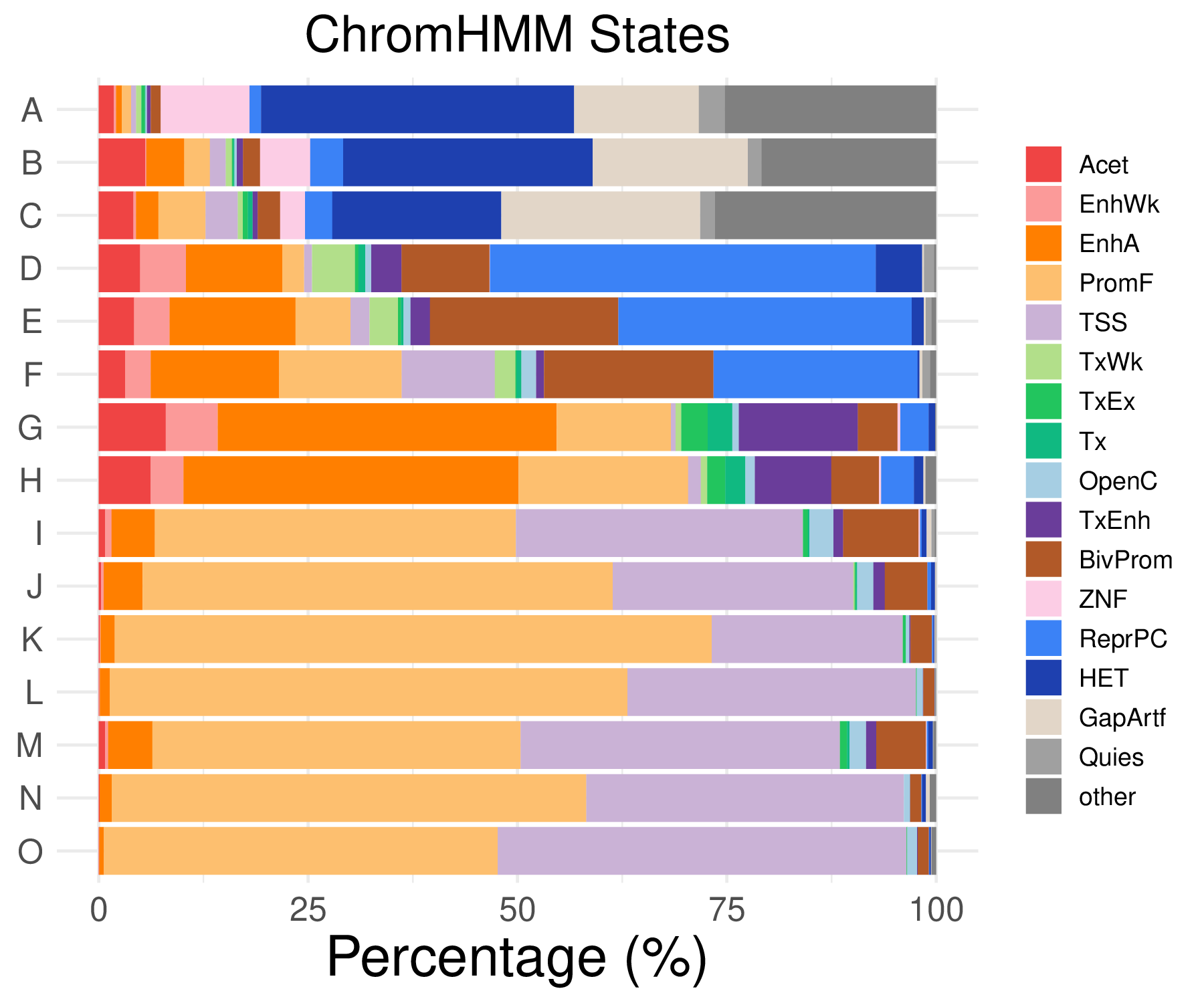
- chromHMM distribution
| Acet | EnhWk | EnhA | PromF | TSS | OpenC | |
|---|---|---|---|---|---|---|
| A | 1.80878552971576 | 0.258397932816538 | 0.689061154177433 | 1.11972437553833 | 0.602928509905254 | 0.172265288544358 |
| B | 5.54744525547445 | 0.145985401459854 | 4.52554744525547 | 3.06569343065693 | 1.8978102189781 | 0.291970802919708 |
| C | 4.15430267062314 | 0.29673590504451 | 2.67062314540059 | 5.6379821958457 | 3.85756676557863 | 0 |
| D | 4.94652406417112 | 5.48128342245989 | 11.4973262032086 | 2.60695187165775 | 0.935828877005348 | 0.735294117647059 |
| TxEnh | BivProm | TxWk | TxEx | Tx | |
|---|---|---|---|---|---|
| A | 0.430663221360896 | 1.20585701981051 | 0.602928509905254 | 0.430663221360896 | 0.0861326442721792 |
| B | 0.72992700729927 | 2.04379562043796 | 0.72992700729927 | 0.145985401459854 | 0.145985401459854 |
| C | 0.593471810089021 | 2.67062314540059 | 0.593471810089021 | 0.593471810089021 | 0.593471810089021 |
| D | 3.6096256684492 | 10.4946524064171 | 5.14705882352941 | 0.401069518716578 | 0.802139037433155 |
| ZNF | ReprPC | HET | GapArtf | Quies | other | |
|---|---|---|---|---|---|---|
| A | 10.594315245478 | 1.37812230835487 | 37.3815676141258 | 14.900947459087 | 3.10077519379845 | 25.2368647717485 |
| B | 5.98540145985401 | 3.94160583941606 | 29.7810218978102 | 18.5401459854015 | 1.60583941605839 | 20.8759124087591 |
| C | 2.9673590504451 | 3.26409495548961 | 20.1780415430267 | 23.7388724035608 | 1.78041543026706 | 26.4094955489614 |
| D | 0.0668449197860962 | 46.0561497326203 | 5.54812834224599 | 0.200534759358289 | 1.20320855614973 | 0.267379679144385 |
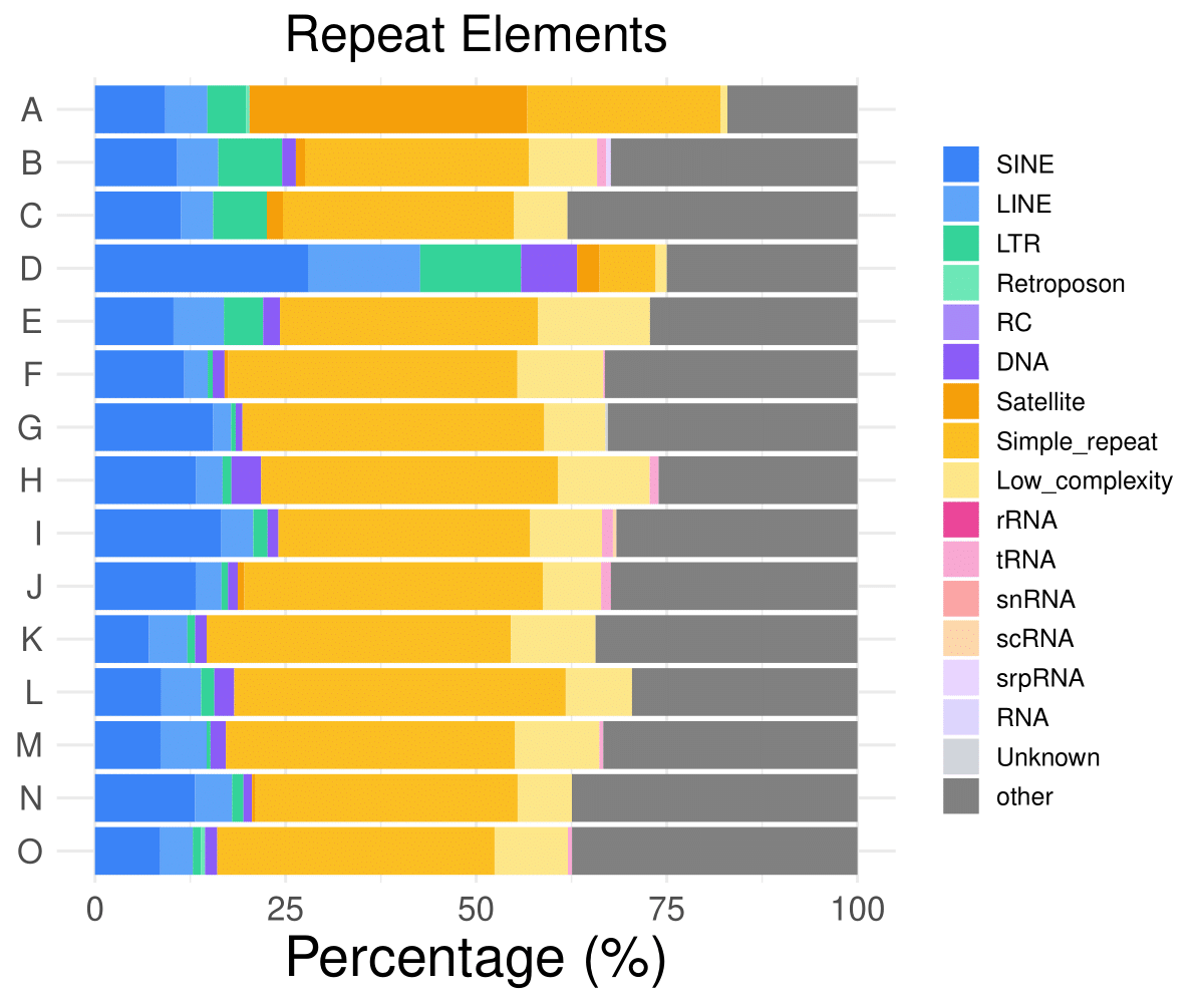
- Repeat distribution
| SINE | LINE | LTR | Retroposon | RC | DNA | |
|---|---|---|---|---|---|---|
| A | 13.5228251507321 | 6.45994832041344 | 22.3083548664944 | 1.98105081826012 | 0 | 1.03359173126615 |
| B | 8.9051094890511 | 5.98540145985401 | 22.3357664233577 | 2.33576642335766 | 0 | 1.16788321167883 |
| C | 8.30860534124629 | 5.6379821958457 | 11.5727002967359 | 2.07715133531157 | 0 | 0.29673590504451 |
| D | 20.5882352941176 | 13.2352941176471 | 9.49197860962567 | 0 | 0 | 5.01336898395722 |
| Satellite | Simple_repeat | Low_complexity | rRNA | tRNA | snRNA | |
|---|---|---|---|---|---|---|
| A | 10.594315245478 | 25.3229974160207 | 0.602928509905254 | 0 | 0 | 0 |
| B | 18.2481751824818 | 20.5839416058394 | 1.45985401459854 | 0.291970802919708 | 0 | 0 |
| C | 23.1454005934718 | 29.080118694362 | 1.78041543026706 | 0.29673590504451 | 0 | 0 |
| D | 0.200534759358289 | 12.9679144385027 | 2.54010695187166 | 0.0668449197860962 | 0 | 0 |
| scRNA | srpRNA | RNA | Unknown | other | |
|---|---|---|---|---|---|
| A | 0 | 0 | 0 | 0.0861326442721792 | 18.0878552971576 |
| B | 0 | 0 | 0 | 0 | 18.6861313868613 |
| C | 0 | 0 | 0 | 0 | 17.8041543026706 |
| D | 0 | 0 | 0 | 0.200534759358289 | 35.6951871657754 |
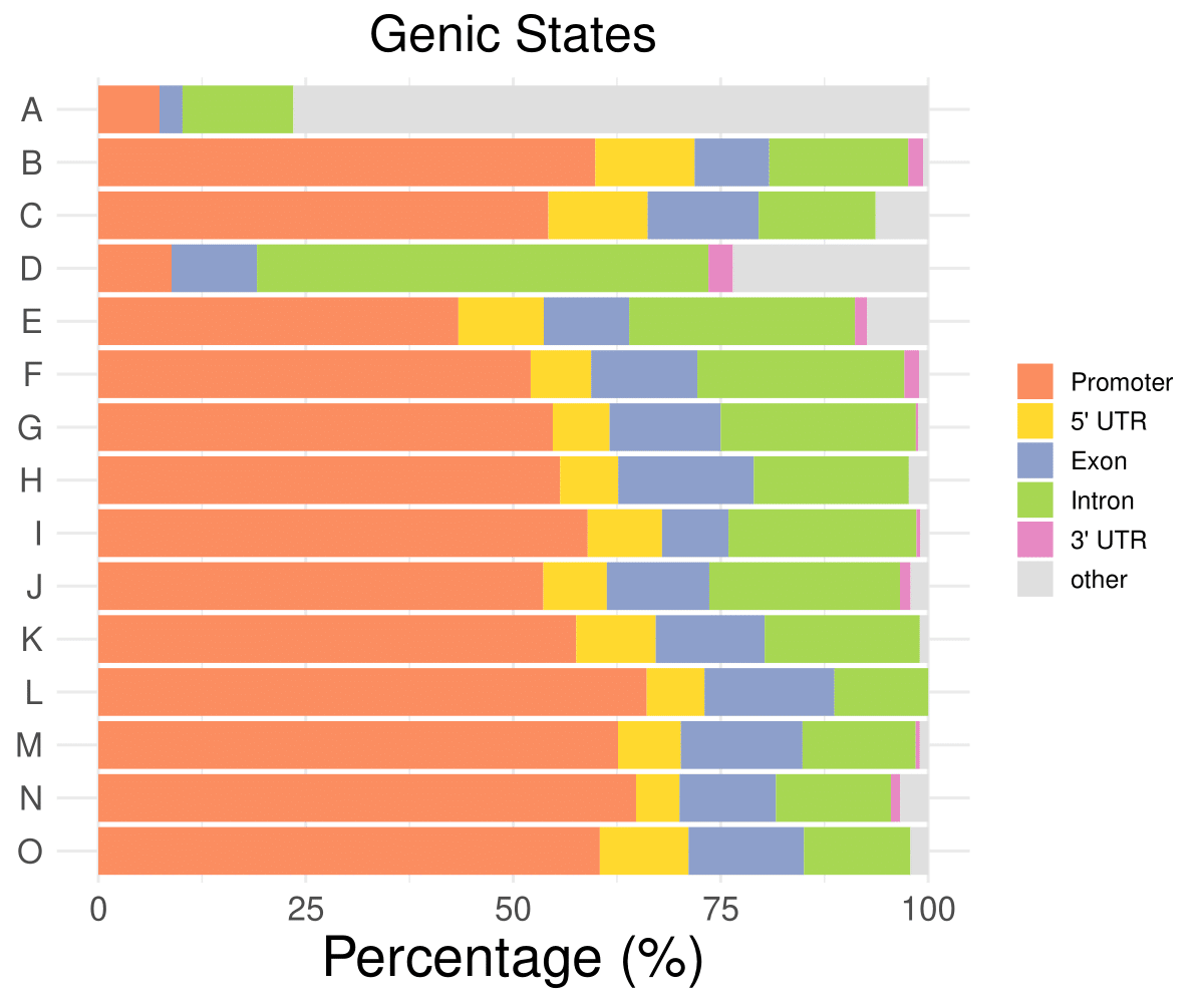
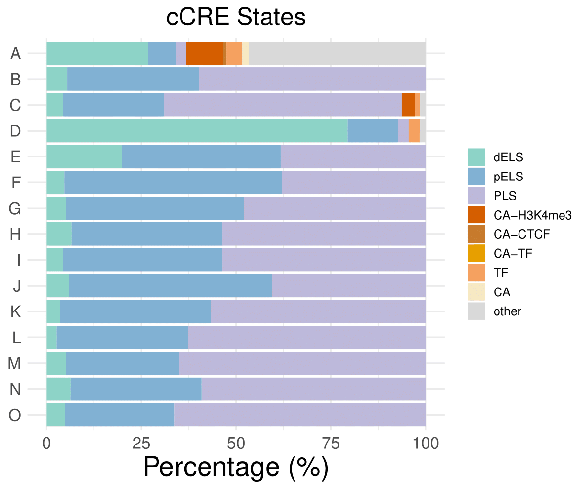
- Cmposition bar plot -
{genic/ccre/chromhmm/repeat}_distribution.pdf- Stacked horizontal bar plot showing ChromHMM chromatin state distribution across clusters
- X-axis: Percentage (0-100%)
- Y-axis: Cluster labels (top to bottom)
Example Usage
library(multiEpiCore)
# Test Data
bi_dir <- "./bicluster"
out_dir <- file.path(bi_dir, "genomic_distribution")
row_cluster_file_path <- file.path(bi_dir, "row_table.tsv")
clustering_genomic_distribution(row_cluster_file_path = row_cluster_file_path, out_dir = out_dir)
5B. Biclustering TFBS Annotation Pipeline
The clustering_TFBS_enrichment() function provides a
complete, automated workflow for analyzing transcription factor binding
site (TFBS) enrichment across multiple clusters of genomic regions. It
handles the entire pipeline from control region generation to enrichment
testing and visualization.
What this function does:
Reads a file containing clustered genomic regions (e.g., from biclustering analysis)
Generates matched control regions for each cluster using gene-based matching
Performs TFBS enrichment analysis comparing each cluster against controls
Creates heatmap visualizations showing enrichment patterns across clusters
Saves all intermediate and final results to organized output files
Parameters
| Parameter | Type | Default | Description | Example |
|---|---|---|---|---|
row_cluster_file_path
|
character | — |
Path to a tab-delimited file containing clustered regions. The file must
include columns region (formatted as chr_start_end) and
cluster (cluster ID).
|
“bicluster_results.tsv”
|
out_dir
|
character |
“./”
|
Output directory where all results will be saved. |
out_dir = “./TFBS_results/”
|
ref_genome
|
character |
“hg38”
|
Reference genome version. Supported options are “hg38”,
“hg19”, “mm10”, and “mm39”.
|
ref_genome = “mm10”
|
ref_source
|
character |
“knownGene”
|
Gene annotation source used for control region generation. Supported
options are “knownGene” (UCSC knownGene) and
“GENCODE” (GENCODE gene models).
|
ref_source = “GENCODE”
|
control_rep
|
integer |
1
|
Multiplier for control region generation, defining the ratio of control
regions to target regions. For example, setting control_rep =
2 generates twice as many control regions.
|
control_rep = 3
|
regions
|
integer |
800
|
Size in base pairs to which all regions are resized, centered on the original region midpoint. |
regions = 500
|
plot
|
logical |
TRUE
|
Whether to generate heatmap visualizations. If set to
FALSE, only enrichment analysis is performed.
|
plot = FALSE
|
Input File Format:
The cluster file must be tab-delimited with at least two columns: -
region: Genomic coordinates in format “chr_start_end”
(underscore-separated) - cluster: Cluster assignment (e.g.,
“cluster_1”, “group_A”, “bicluster_2”)
Output Files
All output files are saved to the specified out_dir:
- Matched control regions -
all_controls.bed- BED file containing all matched control regions used as background for TFBS enrichment analysis
- Regions are combined across clusters and de-duplicated to avoid redundant counting
| chr | start | end | |
|---|---|---|---|
| 1 | chr22 | 17943784 | 17944584 |
| 2 | chr22 | 18845683 | 18846483 |
| 3 | chr22 | 21025481 | 21026281 |
| 4 | chr22 | 21466688 | 21467488 |
| 5 | chr22 | 21665299 | 21666099 |
| 6 | chr22 | 21735986 | 21736786 |
| 7 | chr22 | 21909073 | 21909873 |
| 8 | chr22 | 23754007 | 23754807 |
| 9 | chr22 | 23802581 | 23803381 |
| 10 | chr22 | 24694313 | 24695113 |
- Cluster-level TFBS enrichment table -
TFBS_enrichment_<cluster_label>.tsv
- Per-cluster transcription factor binding site enrichment results
- Includes odds ratio, p-value, FDR, and hit counts for each TF motif
| feature | target_hit | control_hit | target_off | control_off | odds_ratio | pvalue | odds_ratio_se | FDR |
|---|---|---|---|---|---|---|---|---|
| ZNF280A | 88 | 48 | 1073 | 15149 | 25.5991560215223 | 6.4330507582669e-68 | 0.180668823039859 | 1.98781268430447e-65 |
| CBX5 | 94 | 146 | 1067 | 15051 | 9.10598553014674 | 1.37357899538723e-46 | 0.135394988163879 | 2.12217954787327e-44 |
| SETDB1 | 110 | 235 | 1051 | 14962 | 6.68822092373858 | 4.23074725190926e-44 | 0.119430728895671 | 4.35766966946654e-42 |
| TRIM28 | 142 | 568 | 1019 | 14629 | 3.60401724437306 | 3.70986223361873e-31 | 0.0989910152190067 | 2.86586857547047e-29 |
| XRCC3 | 35 | 19 | 1126 | 15178 | 24.2283993097457 | 5.40846255848119e-28 | 0.280590394912017 | 3.34242986114137e-26 |
Note: This table shows annotation results for cluster A in the test dataset.
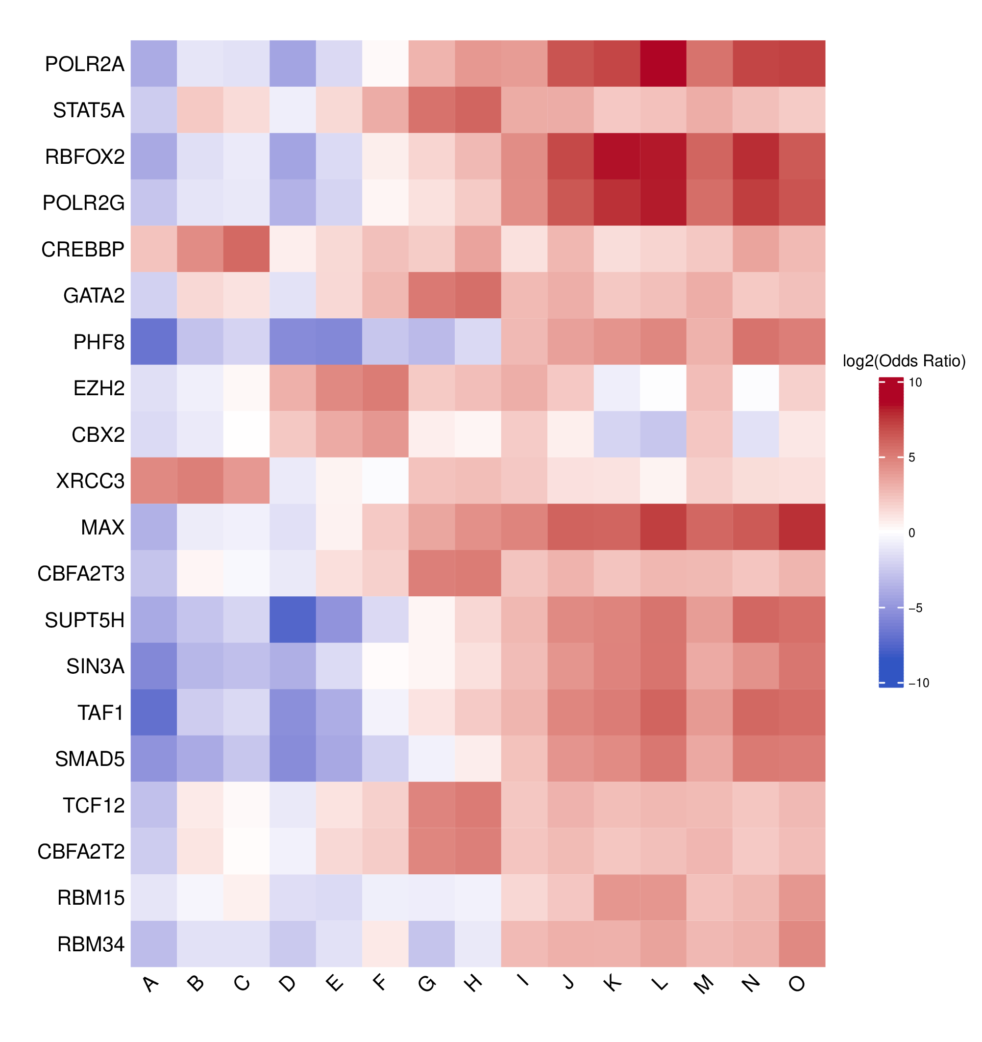
- Full TFBS enrichment heatmap -
TFBS_heatmap_all.pdf(ifplot = TRUE)- Heatmap visualization of enriched TFBS across all clusters
- Log2-transformed odds ratios with a symmetric color scale
- Rows: TFBS
- Columns: Cluster labels

- Top N TFBS heatmap -
TFBS_enrichment_top<n>.pdf(iftop_nprovided andplot = TRUE)- Heatmap showing the top N TFBS with the highest coefficient of variation across clusters
- Highlights TFBS exhibiting the greatest variability between clusters
- Uses the same log2 odds ratio color scale as the full heatmap for consistency
- Rows: TFBS
- Columns: Cluster labels
- Log2 odds ratio matrix -
odds_ratio_log2.csv(ifplot = TRUE)- Matrix of log2-transformed odds ratios for all TFBS × clusters
- Numerical data underlying the TFBS enrichment heatmap
- Rows: TFBS
- Columns: Cluster labels
- FDR matrix -
FDR.csv(ifplot = TRUE)- Matrix of FDR-adjusted p-values for all TFBS × clusters
- Same row and column order as
odds_ratio_log2.csv
Example Usage
library(multiEpiCore)

# Basic usage - complete pipeline with visualization
clustering_TFBS_enrichment(
  row_cluster_file_path = "NMF_clusters.tsv",
  out_dir = "./TFBS_analysis/",
  ref_genome = "hg38"
)

# Custom region size for enhancer analysis
clustering_TFBS_enrichment(
  row_cluster_file_path = "enhancer_clusters.tsv",
  out_dir = "./enhancer_TFBS/",
  ref_genome = "hg38",
  regions = 1000
)

# Mouse genome analysis
clustering_TFBS_enrichment(
  row_cluster_file_path = "mouse_peaks_clustered.tsv",
  out_dir = "./mouse_TFBS/",
  ref_genome = "mm10",
  regions = 500
)

# Generate 3x more control regions for more robust statistics
clustering_TFBS_enrichment(
  row_cluster_file_path = "ATAC_peaks_clustered.tsv",
  out_dir = "./ATAC_TFBS/",
  ref_genome = "hg38",
  control_rep = 3,
  regions = 800
)

# Enrichment analysis only (no heatmap)
clustering_TFBS_enrichment(
  row_cluster_file_path = "clusters.tsv",
  out_dir = "./TFBS_tables/",
  ref_genome = "hg38",
  plot = FALSE
)

# Test Data
bi_dir <- "./bicluster"
out_dir <- file.path(bi_dir, "TFBS_enrichment")
row_cluster_file_path <- file.path(bi_dir, "row_table.tsv")
clustering_TFBS_enrichment(row_cluster_file_path = row_cluster_file_path, out_dir = out_dir)